IMU Sensor Fusion 3D

In this article, the combination of accelerometer and gyroscope data for angle and angular velocity estimation in the 3D case is discussed. Again, there are a lot of online references available on this topic, you may want to take a look at https://www.olliw.eu/2013/imu-data-fusing/ and the many references cited therein.

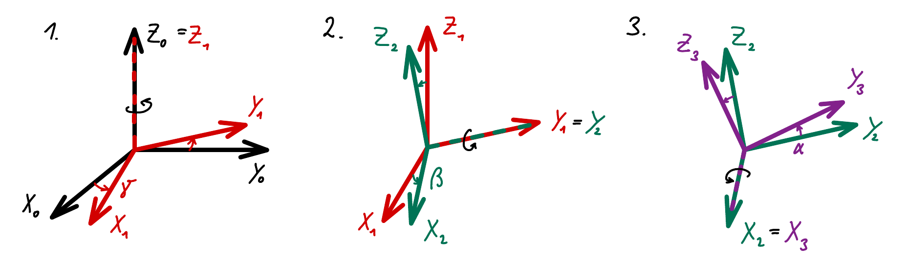
There are different ways to describe rotations in 3D space, well known are e.g. Euler angles and Tait–Bryan angles. For both of them, different axes conventions and orders of rotations about the axes are in use. So first, let us establish a convention for the present article. We use a version of Tait–Bryan angles and refer to the angels by roll, pitch and yaw, for which the symbols \(\alpha\), \(\beta\) and \(\gamma\) are used. These angles describe the orientation of the IMU-fixed coordinate system (with axis \(X_3,Y_3,Z_3\)) with respect to an inertial frame of reference (with axis \(X_0,Y_0,Z_0\)) by the following order of rotations:

rotation by the yaw angle \(\gamma\) about the \(Z_0\)-axis (resulting in an “intermediate” coordinate system with axis \(X_1,Y_1,Z_1\))
rotation by the pitch angle \(\beta\) about the new \(Y_1\)-axis (resulting in an “intermediate” coordinate system with axis \(X_2,Y_2,Z_2\))
rotation by the roll angle \(\alpha\) about the new \(X_2\)-axis (resulting in the “final” coordinate system with axis \(X_3,Y_3,Z_3\))

i.e., the rotation are intrinsic, which means that the rotations are performed around the axes of a coordinate system that changes orientation after each rotation (rather than extrinsic rotations, which are performed around the axes of a fixed coordinate system).

The following figure illustrates the axis- and angle convention just described and used throughout this article.

The rotation matrices for the three elementary rotations are

\[\begin{align} {_0R_1}&=\begin{bmatrix} \cos(\gamma)&-\sin(\gamma)&0\\ \sin(\gamma)&\cos(\gamma)&0\\ 0&0&1 \end{bmatrix} \end{align}\] \[\begin{align} {_1R_2}&=\begin{bmatrix} \cos(\beta)&0&\sin(\beta)\\ 0&1&0\\ -\sin(\beta)&0&\cos(\beta) \end{bmatrix} \end{align}\] \[\begin{align} {_2R_3}&=\begin{bmatrix} 1&0&0\\ 0&\cos(\alpha)&-\sin(\alpha)\\ 0&\sin(\alpha)&\cos(\alpha) \end{bmatrix} \end{align}\]

and for the rotation matrix from the IMU-fixed “3”-system to the initial “0”-system we obtain

\[\begin{align} {_0R_3}&= {_0R_1}~{_1R_2}~{_2R_3}=\tiny{\begin{bmatrix} \cos(\beta)\cos(\gamma)&\sin(\alpha)\sin(\beta)\cos(\gamma)-\sin(\gamma)\cos(\alpha)&\sin(\alpha)\sin(\gamma)+\sin(\beta)\cos(\alpha)\cos(\gamma)\\ \sin(\gamma)\cos(\beta)&\sin(\alpha)\sin(\beta)\cos(\gamma)+\cos(\alpha)\cos(\gamma)&-\sin(\alpha)\cos(\gamma)+\sin(\beta)\sin(\gamma)\cos(\alpha)\\ -\sin(\beta)&\sin(\alpha)\cos(\beta)&\cos(\alpha)\cos(\beta) \end{bmatrix}}\,. \end{align}\]

The meaning of the rotation matrix \({_0R_3}\) (or analogously any other rotation matrix considered here) can be explained as follows. Given a vector \(v\), let \({_3v}\) be its coordinate representation with respect to the IMU-fixed “3”-system. Then its coordinate representation with respect to the initial “0”-system is given by \({_0v}={_0R_3}~{_3v}\). Conversely, \({_3v}={_3R_0}~{_0v}\) with \({_3R_0}={_0R_3}^{-1}={_0R_3}^T\).

We can use the results obtained so far for deriving relations between the accelerations measured by the IMU due to gravity and the angles which describe the orientation of the IMU-fixed “3”-system with respect to the initial “0”-system. In the initial “0”-system, we have the “gravitation vector”

\[\begin{align} {_0g}&=\begin{bmatrix} 0\\ 0\\ -g \end{bmatrix}\,. \end{align}\]

Let \(acc_X, acc_Y, acc_Z\) be the accelerations measured by the IMU along the axes \(X_3,Y_3,Z_3\) of its reference frame. When only gravity is acting on the IMU, but no additional translatory accelerations, then the accelerations measured by the IMU are (despite from measurement noise and disturbances) only caused by gravity, i.e., we have

\[\begin{align} {_3acc}:=\begin{bmatrix} acc_X\\ acc_Y\\ acc_Z \end{bmatrix}=-{_3g}=-{_3R_0}~{_0g}=\begin{bmatrix} -g\sin(\beta)\\ g\sin(\alpha)\cos(\beta)\\ g\cos(\alpha)\cos(\beta) \end{bmatrix} \end{align}\label{eq:acc}\tag{1}\]

(The reason for the minus after the second equals sign is that the IMU shows a positive acceleration in each axis which points against the direction of the \(g\) vector. E.g. when all angles are zero, the \(g\) vector points against the \(Z_3\) axis and thus the IMU reading is \(acc_Z=g\)). From (\ref{eq:acc}), we immediately obtain the equations

\[\begin{align} \tan(\alpha)&=\frac{acc_Y}{acc_Z}\\ \sin(\beta)&=-\frac{acc_X}{\sqrt{acc_X^2+acc_Y^2+acc_Z^2}} \end{align}\]

and when restricting the roll and pitch angle to \(-\pi/2\leq\alpha,\beta\leq\pi/2\) we obtain

\[\begin{align} \alpha&=\arctan\left(\frac{acc_Y}{acc_Z}\right)=\arcsin\left(\frac{acc_Y}{\sqrt{acc_Y^2+acc_Z^2}}\right)\\ \beta&=-\arcsin\left(\frac{acc_X}{\sqrt{acc_X^2+acc_Y^2+acc_Z^2}}\right)\,. \end{align}\label{eq:alpha_beta_acc}\tag{2}\]

The accelerometer data can thus be used for calculating the roll angle \(\alpha\) and the pitch angle \(\beta\), but it does not provide any information about the yaw angle \(\gamma\).

Next, let us derive a relation between the rates of change of the roll-, pitch- and yaw angle, denoted by \(\dot{\alpha},\dot{\beta},\dot{\gamma}\) and the angular velocities \(\omega_X,\omega_Y,\omega_Z\) measured by the IMU in its reference frame. Recall the order of rotations

rotation by yaw angle \(\gamma\) about the \(Z_0\)-axis (resulting in an “intermediate” coordinate system with axis \(X_1,Y_1,Z_1\))
rotation by the pitch angle \(\beta\) about the new \(Y_1\)-axis (resulting in an “intermediate” coordinate system with axis \(X_2,Y_2,Z_2\))
rotation by the roll angle \(\alpha\) about the new \(X_2\)-axis (resulting in the “final” coordinate system with axis \(X_3,Y_3,Z_3\))

The roll rotation is an elementary rotation about the \(X_2\)-axis, which thus always aligns with the IMU-fixed \(X_3\)-axis. Therefore, the contribution of \(\dot{\alpha}\) to the angular velocity vector \(\omega\) which the IMU measures, is simply given by

\[\begin{align} {_3\omega_{\dot{\alpha}}}=\begin{bmatrix} \dot{\alpha}\\ 0\\ 0 \end{bmatrix} \end{align}\]

Similarly, the pitch rotation is an elementary rotation about the \(Y_1\)-axis. The \(Y_1\)-axis aligns with the \(Y_2\)-axis. Therefore,

\[\begin{align} {_2\omega_{\dot{\beta}}}=\begin{bmatrix} 0\\ \dot{\beta}\\ 0 \end{bmatrix} \end{align}\]

and in turn

\[\begin{align} {_3\omega_{\dot{\beta}}}&={_3R_2}~{_2\omega_{\dot{\beta}}}=\begin{bmatrix} 0\\ \dot{\beta}\cos(\alpha)\\ -\dot{\beta}\sin(\alpha) \end{bmatrix}\,. \end{align}\]

Finally, the yaw rotation is an elementary rotation about the \(Z_0\)-axis. The \(Z_0\)-axis aligns with the \(Z_1\)-axis. Therefore,

\[\begin{align} {_1\omega_{\dot{\gamma}}}=\begin{bmatrix} 0\\ 0\\ \dot{\gamma} \end{bmatrix} \end{align}\]

and in turn

\[\begin{align} {_3\omega_{\dot{\gamma}}}&={_3R_2}~{_2R_1}~{_1\omega_{\dot{\gamma}}}=\begin{bmatrix} -\dot{\gamma}\sin(\beta)\\ \dot{\gamma}\sin(\alpha)\cos(\beta)\\ \dot{\gamma}\cos(\alpha)\cos(\beta) \end{bmatrix}\,. \end{align}\]

In total, the angular velocity measured by the IMU is thus (despite from measurement noise and disturbances)

\[\begin{align} {_3\omega}&=\begin{bmatrix} \omega_X\\ \omega_Y\\ \omega_Z \end{bmatrix}={_3\omega_{\dot{\alpha}}}+{_3\omega_{\dot{\beta}}}+{_3\omega_{\dot{\gamma}}}=\begin{bmatrix} \dot{\alpha}-\dot{\gamma}\sin(\beta)\\ \dot{\beta}\cos(\alpha)+\dot{\gamma}\sin(\alpha)\cos(\beta)\\ -\dot{\beta}\sin(\alpha)+\dot{\gamma}\cos(\alpha)\cos(\beta) \end{bmatrix}\,. \end{align}\label{eq:omega}\tag{3}\]

From (\ref{eq:omega}), we directly obtain the following relation between the rates of change \(\dot{\alpha},\dot{\beta},\dot{\gamma}\) of roll, pitch and yaw, and the angular velocities \(\omega_X,\omega_Y,\omega_Z\) measured by the IMU in its reference frame

\[\begin{align} \dot{\alpha}&=\omega_X+(\omega_Y\sin(\alpha)+\omega_Z\cos(\alpha))\tan(\beta)\\ \dot{\beta}&=\omega_Y\cos(\alpha)-\omega_Z\sin(\alpha)\\ \dot{\gamma}&=(\omega_Y\sin(\alpha)+\omega_Z\cos(\alpha))/\cos(\beta)\,. \end{align}\label{eq:alpha_p_beta_p_gamma_p}\tag{4}\]

Observer Based Orientation Estimation

The equations (\ref{eq:alpha_beta_acc}) and (\ref{eq:alpha_p_beta_p_gamma_p}) represent the ideal case of an IMU without any measurement noise or inaccuracies. In the following we take into account that the angles calculated from the IMU’s accelerometer data via (\ref{eq:alpha_beta_acc}) can slightly deviate from the actual ones and that the angular velocities measured by the IMU can slightly deviate from the actual ones. This leads to the following model of the IMU

\[\begin{align} \dot{\alpha}&=\omega_{X,gyro}+(\omega_{Y,gyro}\sin(\alpha)+\omega_{Z,gyro}\cos(\alpha))\tan(\beta)+v_1\\ \dot{\beta}&=\omega_{Y,gyro}\cos(\alpha)-\omega_{Z,gyro}\sin(\alpha)+v_2\\ \dot{\gamma}&=(\omega_{Y,gyro}\sin(\alpha)+\omega_{Z,gyro}\cos(\alpha))/\cos(\beta)+v_3\\ \alpha_{acc}&=\alpha+n_1\\ \beta_{acc}&=\beta+n_2\,, \end{align}\label{eq:model_continous}\tag{5}\]

where we have replaced the actual angular velocities \(\omega_X,\omega_Y,\omega_Z\) by the IMU measurements \(\omega_{X,gyro},\omega_{Y,gyro},\omega_{Z,gyro}\) and introduced the disturbances \(v_1,v_2,v_3\) to account for the deviations between actual and measured quantities. Similarly, to take the deviation between the actual angles \(\alpha,\beta\) and the angles \(\alpha_{acc},\beta_{acc}\) calculated from the IMU’s accelerometer data via (\ref{eq:alpha_beta_acc}) into account, we have introduced the disturbances \(n_1,n_2\). The angles \(\alpha,\beta,\gamma\) in this model still represent the actual roll, pitch and yaw angles, which we aim to estimate. Note however that there is an obvious problem with this model, namely the yaw angle \(\gamma\) in (\ref{eq:model_continous}) is unobservable, which means that the estimate of the yaw angle \(\gamma\) will always drift.

For the applications which I have in mind, the yaw angle estimate is not of importance and since the yaw angle \(\gamma\) does not appear anywhere on the right hand side of (\ref{eq:model_continous}), we can simply omit its equation, which leads to the “reduced” model

\[\begin{align} \dot{\alpha}&=\omega_{X,gyro}+(\omega_{Y,gyro}\sin(\alpha)+\omega_{Z,gyro}\cos(\alpha))\tan(\beta)+v_1\\ \dot{\beta}&=\omega_{Y,gyro}\cos(\alpha)-\omega_{Z,gyro}\sin(\alpha)+v_2\\ \alpha_{acc}&=\alpha+n_1\\ \beta_{acc}&=\beta+n_2 \end{align}\label{eq:model_continous_reduced}\tag{6}\]

for pitch- and roll angle estimation. In regard of a practical realization of the observer which we are going to design, let us already discretize the model and then design an observer for the obtained discrete time model. A forward Euler discretization of (\ref{eq:model_continous_reduced}) with sampling time \(T_s\) yields

\[\begin{align} \alpha_{k+1}&=\small{\alpha_k+T_s(\omega_{X,gyro,k}+(\omega_{Y,gyro,k}\sin(\alpha_k)+\omega_{Z,gyro,k}\cos(\alpha_k))\tan(\beta_k))+v_{1,k}}\\ \beta_{k+1}&=\beta_k+T_s(\omega_{Y,gyro,k}\cos(\alpha_k)-\omega_{Z,gyro,k}\sin(\alpha_k))+v_{2,k}\\ \alpha_{acc,k}&=\alpha_k+n_{1,k}\\ \beta_{acc,k}&=\beta_k+n_{2,k}\,, \end{align}\label{eq:model_discrete_reduced}\tag{7}\]

where for simplicity, we denote the disturbances of the continuous and the discrete time models by the same symbols and omit the factor \(T_s\) in front of \(v_{1,k}\) and \(v_{2,k}\) which would emerge due to the discretization (i.e., we assume that this factor is already included in \(v_{1,k}\) and \(v_{2,k}\)). By defining

\[\begin{align} x_k&=\begin{bmatrix} x_{1,k}\\ x_{2,k} \end{bmatrix}=\begin{bmatrix} \alpha_k\\ \beta_k \end{bmatrix}\,, &u_k&=\begin{bmatrix} u_{1,k}\\ u_{2,k}\\ u_{3,k} \end{bmatrix}=\begin{bmatrix} \omega_{X,gyro,k}\\ \omega_{Y,gyro,k}\\ \omega_{Z,gyro,k} \end{bmatrix}\,, &v_k&=\begin{bmatrix} v_{1,k}\\ v_{2,k} \end{bmatrix}\,, \end{align}\] \[\begin{align} y_k&=\begin{bmatrix} y_{1,k}\\ y_{2,k} \end{bmatrix}=\begin{bmatrix} \alpha_{acc,k}\\ \beta_{acc,k} \end{bmatrix}\,, &n_k&=\begin{bmatrix} n_{1,k}\\ n_{2,k} \end{bmatrix} \end{align}\]

as well as

\[\begin{align} f(x_k,u_k)&=\begin{bmatrix} x_{1,k}+T_s(u_{1,k}+(u_{2,k}\sin(x_{1,k})+u_{3,k}\cos(x_{1,k}))\tan(x_{2,k}))\\ x_{2,k}+T_s(u_{2,k}\cos(x_{1,k})-u_{3,k}\sin(x_{1,k})) \end{bmatrix} \end{align}\]

and

\[\begin{align} h(x_k)&=\begin{bmatrix} x_{1,k}\\ x_{2,k} \end{bmatrix} \end{align}\]

this model can be written in the form

\[\begin{align} x_{k+1}&=f(x_k,u_k)+v_k\\ y_k&=h(x_k)+n_k\,, \end{align}\label{eq:model_discrete_standard_notation}\tag{8}\]

which is the usual notation for a nonlinear time-invariant discrete time model subject to process noise \(v_k\) and measurement noise \(n_k\). Under the assumption that the process noise and the measurement noise are both zero mean multivariate Gaussian noises (which we assume here due to lack of a more reasonable assumption), the model (\ref{eq:model_discrete_standard_notation}) meets the requirements for designing an extended Kalman filter (EKF) for estimating its state. The state estimation by the EKF algorithm works as follows:

In step \(k\), we have estimates \(\hat{x}_{k\vert k-1}\) for the state and covariance matrix \(P_{k\vert k-1}\) for step \(k\) based on the data up to step \(k-1\) (indicated by the notation \(k\vert k-1\)). Additionally, in step \(k\), the input \(u_k\) (in our case gyro measurements) and output \(y_k\) (in our case calculated from accelerometer measurements) are available. The first step is to use \(y_k\) for calculating the a posteriori estimates \(\hat{x}_{k\vert k}\) and \(P_{k\vert k}\) for step \(k\) from the given a priori estimates \(\hat{x}_{k\vert k-1}\) and \(P_{k\vert k-1}\):

\[\begin{align} C_k&=\frac{\partial h(x_k)}{\partial x_k}{\large\vert_{\hat{x}_{k\vert k-1}}}\\ L_k&=P_{k\vert k-1} C_k^T (C_k P_{k\vert k-1} C_k^T+R_k)^{-1}\\ \hat{x}_{k\vert k}&=\hat{x}_{k\vert k-1}+L_k(y_k-h(\hat{x}_{k\vert k-1}))\\ P_{k\vert k}&=(I-L_kC_k)P_{k\vert k-1} \end{align}\]

Next, the a posteriori estimates \(\hat{x}_{k\vert k}\) and \(P_{k\vert k}\) are used for calculating a priori estimates for the step \(k+1\):

\[\begin{align} A_k&=\frac{\partial f(x_k,u_k)}{\partial x_k}{\large\vert_{\hat{x}_{k\vert k},u_k}}\\ \hat{x}_{k+1\vert k}&=f(\hat{x}_{k\vert k},u_k)\\ P_{k+1\vert k}&=A_k P_{k\vert k} A_k^T+Q_k \end{align}\]

The matrices \(Q_k\) and \(R_k\) in the above equations represent the covariance matrices of the process noise \(v_k\) and measurement noise \(n_k\) (which we from now on assume to be constant, i.e., \(Q_k=Q\) and \(R_k=R\)). The procedure consists of a correct- and a predict step. We initialize with \(\hat{x}_{0\vert -1}=x_0\) and \(P_{0\vert -1}=0\) if the initial state is known, otherwise we may initialize with \(\hat{x}_{0\vert -1}=0\) and \(P_{0\vert -1}=\lambda I\) with \(\lambda>>1\). The first correct step takes into account \(y_0\) (in our case the angles calculated from the accelerometer measurements taken in step \(k=0\)) to calculate improved estimates for step \(k=0\), namely \(\hat{x}_{0\vert 0}\) and \(P_{0\vert 0}\). In the predict step, the improved estimates and \(u_0\) (in our case the gyro measurements taken in step \(k=0\)) are used for pre-calculating estimates \(\hat{x}_{1\vert 0}\) and \(P_{1\vert 0}\) for step \(k=1\), which are then in step \(k=1\), when \(y_1\) and \(u_1\) are available, improved to \(\hat{x}_{1\vert 1}\) and \(P_{1\vert 1}\) and advanced to \(\hat{x}_{2\vert 1}\) and \(P_{2\vert 1}\) for step \(k=2\), etc. The improved estimates, i.e., those in which the subscripts match, are intended for further use, e.g. in a flight control algorithm.

The tuning parameters of the EKF are the covariance matrices \(Q_k\) and \(R_k\) (resp. \(Q\) and \(R\) when we assume that they are constant). Those must be positive (semi)definite matrices and when lacking a better guess, we may simply choose diagonal matrices for them. In a nutshell, a large entry in \(Q\), resp. \(R\), means that the corresponding component of \(v\), resp. \(n\), in the model (\ref{eq:model_discrete_standard_notation}) has large variance, which in turn means that we have little trust in the corresponding model equation, resp. measurement. For a good smoothing of \(\alpha_{acc}\) and \(\beta_{acc}\) calculated from the usually quite noisy accelerometer data, large values in \(R\) compared to \(Q\) are required. On the other hand, going to extreme, i.e., trusting the model equations too much can lead to instability.

Practical Implementation

Below is some c code which implements the EKF algorithm from above for the model (\ref{eq:model_discrete_reduced}). For this particular model, the equations for the correct step are

\[\begin{align} \begin{bmatrix}l_k^{11}&l_k^{12}\\ l_k^{21}&l_k^{22}\end{bmatrix}&=\begin{bmatrix}p_{k\vert k-1}^{11}&p_{k\vert k-1}^{12}\\ \ast &p_{k\vert k-1}^{22}\end{bmatrix}\left(\begin{bmatrix}p_{k\vert k-1}^{11}&p_{k\vert k-1}^{12}\\ \ast &p_{k\vert k-1}^{22}\end{bmatrix}+\begin{bmatrix}r^{11}& r^{12}\\ \ast & r^{22}\end{bmatrix}\right)^{-1}\\ \begin{bmatrix}\hat{\alpha}_{k\vert k}\\ \hat{\beta}_{k\vert k}\end{bmatrix}&=\begin{bmatrix}\hat{\alpha}_{k\vert k-1}\\ \hat{\beta}_{k\vert k-1}\end{bmatrix}+\begin{bmatrix}l_k^{11}&l_k^{12}\\ l_k^{21}&l_k^{22}\end{bmatrix}\begin{bmatrix}\alpha_{acc,k}-\hat{\alpha}_{k\vert k-1}\\ \beta_{acc,k}-\hat{\beta}_{k\vert k-1}\end{bmatrix}\\ \begin{bmatrix}p_{k\vert k}^{11}&p_{k\vert k}^{12}\\ \ast &p_{k\vert k}^{22}\end{bmatrix}&=\left(\begin{bmatrix}1& 0\\0& 1\end{bmatrix}-\begin{bmatrix}l_k^{11}&l_k^{12}\\ l_k^{21}&l_k^{22}\end{bmatrix}\right)\begin{bmatrix}p_{k\vert k-1}^{11}&p_{k\vert k-1}^{12}\\ \ast &p_{k\vert k-1}^{22}\end{bmatrix} \end{align}\]

and the equations for the update step are

\[\begin{align} \begin{bmatrix}a_k^{11}& a_k^{12}\\ a_k^{21}& a_k^{22}\end{bmatrix}&=\tiny{\begin{bmatrix}1+T_s(\omega_{Y,gyro,k}\cos(\alpha_{k\vert k})-\omega_{Z,gyro,k}\sin(\alpha_{k\vert k})\tan{\beta_{k\vert k}})& T_s(\omega_{Y,gyro,k}\sin(\alpha_{k\vert k})+\omega_{Z,gyro,k}\cos(\alpha_{k\vert k}))(1+\tan(\beta_{k\vert k}))\\ T_s(-\omega_{Y,gyro,k}\sin(\alpha_{k\vert k}-\omega_{Z,gyro,k}\cos(\alpha_{k\vert k}))) & 1\end{bmatrix}}\\ \begin{bmatrix}\hat{\alpha}_{k+1\vert k}\\ \hat{\beta}_{k+1\vert k}\end{bmatrix}&=\small{\begin{bmatrix}\hat{\alpha}_{k\vert k}+T_s(\omega_{X,gyro,k}+(\omega_{Y,gyro,k}\sin(\hat{\alpha}_{k\vert k})+\omega_{Z,gyro,k}\cos(\hat{\alpha}_{k\vert k}))\tan(\hat{\beta}_{k\vert k}))\\ \hat{\beta}_{k\vert k}+T_s(\omega_{Y,gyro,k}\cos(\hat{\alpha}_{k\vert k})-\omega_{Z,gyro,k}\sin(\hat{\alpha}_{k\vert k}))\end{bmatrix}}\\ \begin{bmatrix}p_{k+1\vert k}^{11}&p_{k+1\vert k}^{12}\\ \ast &p_{k+1\vert k}^{22}\end{bmatrix}&=\begin{bmatrix}a_k^{11}& a_k^{12}\\ a_k^{21}& a_k^{22}\end{bmatrix} \begin{bmatrix}p_{k\vert k}^{11}&p_{k\vert k}^{12}\\ \ast &p_{k\vert k}^{22}\end{bmatrix} \begin{bmatrix}a_k^{11}& a_k^{21}\\ a_k^{12}& a_k^{22}\end{bmatrix}+\begin{bmatrix}q^{11}& q^{12}\\ \ast & q^{22}\end{bmatrix}\,. \end{align}\]

The covariance matrix \(P\) is initialized as a symmetric matrix and it can be shown that it stays symmetric throughout the iterations. Also the covariance matrices \(Q\) and \(R\) are symmetric, and thus, all these matrices have only \(3\) independent elements, as indicated in the equations above by the \(\ast\). The code below is a near-direct implementation of the equations presented above. The function takes the roll- and pitch angle calculated via (\ref{eq:alpha_beta_acc}) from the accelerometer data, as well as the gyroscope data as input. Furthermore, two float pointers have to be passed as function arguments. After each iteration, the refefrenced variables hold the filtered roll- and pitch angle, i.e., the output of the EKF. The inputs must be provided in \(\mathrm{rad}\) and \(\mathrm{rad/s}\), the output is also in \(\mathrm{rad}\). The function has to be called periodically such that exactly the sampling time \(T_s\) lies between consecutive calls.

#define TS 10000 // sampling time in micro seconds

/* measurement noise covariance matrix */
#define R11 1.0e3
#define R12 0.0
#define R22 1.0e3

/* process noise covariance matrix */
#define Q11 1.0
#define Q12 0.0
#define Q22 1.0
...

void observer(float alpha_acc_k, float beta_acc_k, float omegaX_gyro_k, float omegaY_gyro_k, 
        float omegaZ_gyro_k, float *alpha, float *beta) {
    static float alpha_k_km1 = 0;
    static float beta_k_km1 = 0;
    static float p11_k_km1 = 0;
    static float p12_k_km1 = 0;
    static float p22_k_km1 = 0;

    /* 1. use input data of step k (alpha_acc_k, beta_acc_k, omegaX_gyro_k, omegaY_gyro_k, omegaZ_gyro_k), 
    for correcting the estimates which were predicted in the previous step based on data up to step k-1 */

    float det = (p11_k_km1+R11)*(p22_k_km1+R22)-(p12_k_km1+R12)*(p12_k_km1+R12);
    float l11 = (p11_k_km1*(p22_k_km1 + R22) - p12_k_km1*(p12_k_km1 + R12))/det;
    float l12 = (-p11_k_km1*R12 + p12_k_km1*R11)/det;
    float l21 = (p12_k_km1*R22 - p22_k_km1*R12)/det;
    float l22 = (-p12_k_km1*(p12_k_km1 + R12) + p22_k_km1*(p11_k_km1 + R11))/det;

    float alpha_k_k = alpha_k_km1 + l11*(alpha_acc_k - alpha_k_km1) + l12*(beta_acc_k - beta_k_km1);
    float beta_k_k = beta_k_km1 + l21*(alpha_acc_k - alpha_k_km1) + l22*(beta_acc_k - beta_k_km1);
    
    float p11_k_k = -l12*p12_k_km1 + p11_k_km1*(1 - l11);
    float p12_k_k = -l12*p22_k_km1 + p12_k_km1*(1 - l11);
    float p22_k_k = -l21*p12_k_km1 + p22_k_km1*(1 - l22);

    /* "return" the corrected estimates */
    *alpha = alpha_k_k;
    *beta = beta_k_k;

    /* 2. preparation for the next step: calculate predictions for step k+1 based on the currently available data up to step k
    (In the current step, they would be called e.g. alpha_kp1_k, but in the next step they are e.g. alpha_k_km1. Since we
    prepare them for the next step, they are already called alpha_k_km1, etc.) */
        
    float sin_alpha = sin(alpha_k_k);
    float cos_alpha = cos(alpha_k_k);
    float tan_beta = tan(beta_k_k);

    float a11 = 1 + TS * 1e-6 * (omegaX_gyro_k + (omegaY_gyro_k * cos_alpha - omegaZ_gyro_k * sin_alpha) * tan_beta);
    float a12 = TS * 1e-6 * (omegaY_gyro_k * sin_alpha + omegaZ_gyro_k * cos_alpha) * (pow(tan_beta,2) + 1);
    float a21 = TS * 1e-6 * (-omegaY_gyro_k * sin_alpha - omegaZ_gyro_k * cos_alpha);
    float a22 = 1;

    alpha_k_km1 = alpha_k_k + TS * 1e-6 * (omegaX_gyro_k + (omegaY_gyro_k * sin_alpha + omegaZ_gyro_k * cos_alpha) * tan_beta);
    beta_k_km1 = beta_k_k + TS * 1e-6 * (omegaY_gyro_k * cos_alpha - omegaZ_gyro_k * sin_alpha);

    p11_k_km1 = a11*(a11*p11_k_k + a12*p12_k_k) + a12*(a11*p12_k_k + a12*p22_k_k) + Q11;
    p12_k_km1 = a21*(a11*p11_k_k + a12*p12_k_k) + a22*(a11*p12_k_k + a12*p22_k_k) + Q12;
    p22_k_km1 = a21*(a21*p11_k_k + a22*p12_k_k) + a22*(a21*p12_k_k + a22*p22_k_k) + Q22;
}

int main() {
    ...
    float alpha_acc = asin(accY/sqrt(accY*accY+accZ*accZ));
    float beta_acc = -asin(accX/sqrt(accX*accX+accY*accY+accZ*accZ));
    float alpha, beta;
    observer(alpha_acc, beta_acc, gyroX, gyroY, gyroZ, &alpha, &beta);
    ...
}

Bias Estimation

Similar to the 1D case, we may drop the assumption that the disturbances \(v_{1,k},v_{2,k}\) in (\ref{eq:model_discrete_reduced}) have zero mean (which was required for the EKF) and instead decompose them into (approximately) constant biases \(b_{1,k},b_{2,k}\) and zero mean remainders \(\tilde{v}_{1,k},\tilde{v}_{2,k}\), i.e., \(v_{1,k}=b_{1,k}+\tilde{v}_{1,k}\) and \(v_{2,k}=b_{2,k}+\tilde{v}_{2,k}\). In order to take these biases into account, the model (\ref{eq:model_discrete_reduced}) is extended to

\[\begin{align} \alpha_{k+1}&=\alpha_k+T_s(\omega_{X,gyro,k}+(\omega_{Y,gyro,k}\sin(\alpha_k)+\omega_{Z,gyro,k}\cos(\alpha_k))\tan(\beta_k))+b_{1,k}+\tilde{v}_{1,k}\\ \beta_{k+1}&=\beta_k+T_s(\omega_{Y,gyro,k}\cos(\alpha_k)-\omega_{Z,gyro,k}\sin(\alpha_k))+b_{2,k}+\tilde{v}_{2,k}\\ b_{1,k+1}&=b_{1,k}+v_{3,k}\\ b_{2,k+1}&=b_{2,k}+v_{4,k}\\ \alpha_{acc,k}&=\alpha_k+n_{1,k}\\ \beta_{acc,k}&=\beta_k+n_{2,k}\,, \end{align}\]

where \(v_{3,k},v_{4,k}\) are again zero mean process noise terms (by which we model the fact that the biases may only be approximately constant). For this model, we can again design an EKF. Note however that the bias estimation here does not directly estimate the biases of the gyro measurements, as it is the case in its 1D counterpart, but rather biases of the whole right hand sides of the equations for \(\alpha_{k+1}\) and \(\beta_{k+1}\). Unfortunately, constant biases of the gyro measurements \(\omega_{Y,gyro}\) and \(\omega_{Z,gyro}\) do NOT cause constant biases of the right hand sides of the equations for \(\alpha_{k+1}\) and \(\beta_{k+1}\), since therein \(\omega_{Y,gyro}\) and \(\omega_{Z,gyro}\) are multiplied by terms which depend on \(\alpha_k\) and \(\beta_k\) and are thus not constant.