
IMU Sensor Fusion
In this article, the combination of accelerometer and gyroscope data for angle and angular velocity estimating is discussed. There are a lot of online references available on this topic, you may want to take a look at https://www.olliw.eu/2013/imu-data-fusing/ and the many references cited therein. The approach discussed in this article is based on an observer. The observer which we are going to design will be able to deal with a large bias of the gyroscope measurement by estimating the bias and using this estimate for correcting the gyroscope measurement.
Throughout this article, only the rotation around a single axis is considered. Hence, angle \(\theta\) and angular velocity \(\omega\) are simply related via
\[\begin{align} \dot{\theta}&=\omega\,. \end{align}\label{eq:theta omega}\tag{1}\]Now consider an IMU (inertial measurement unit) as depicted in Figure 1 and let us only consider rotation around the \(z\)-axis. The IMU measures acceleration in \(x\)- and \(y\)-direction and angular velocity around the \(z\)-axis.
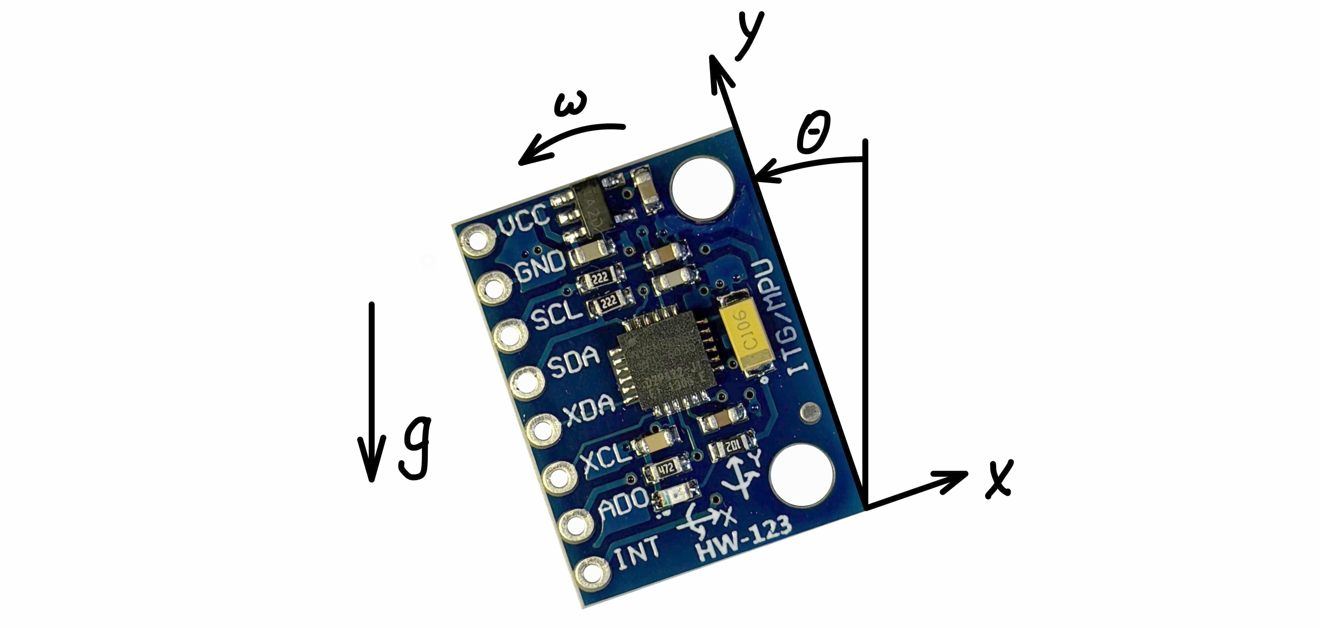
When only gravity is acting on the IMU, but no additional translatory acceleration in \(x\)- or \(y\)-direction, then the accelerations measured by the IMU are (despite from measurement noise and disturbances) \(acc_X=g\sin(\theta)\) and \(acc_Y=g\cos(\theta)\). From the accelerometer data, we thus obtain an estimate for the angle \(\theta\) via
\[\begin{align} \theta_{acc}&=\arctan 2(acc_X,acc_Y)\,. \end{align}\label{eq:theta acc atan2}\tag{2}\]When only angles between \(\pm 90°\) are of interest, then (\ref{eq:theta acc atan2}) can be simplified to
\[\begin{align} \theta_{acc}&=\arctan\left(\tfrac{acc_X}{acc_Y}\right)\,, \end{align}\]or alternatively
\[\begin{align} \theta_{acc}&=\arcsin\left(\tfrac{acc_X}{\sqrt{acc_X^2+acc_Y^2}}\right)\,. \end{align}\]An estimate for the angular velocity \(\omega\) is directly given by the IMU measurement \(\omega_{gyro}\). Integrating \(\omega_{gyro}\) also provides an estimate for the angle \(\theta\). However, due to the integration, this estimate drifts over time, especially, when the gyro measurement has some bias. The estimate \(\theta_{acc}\) obtained from the accelerometer data does not drift, but it is usually very noisy since the accelerometers are very sensitive to vibrations. In order to obtain an estimate for \(\theta\) which does not drift and at the same time is not too noisy, it is thus necessary to appropriately combine \(\omega_{gyro}\) and \(\theta_{acc}\).
Complementary Filter
A common method for combining the gyroscope and the accelerometer measurements is to use a complementary filter. The basic idea of the complementary filter approach is simple: The estimate \(\theta_{acc}\) is noisy, hence it is sent through a low-pass filter. The integrated gyro signal drifts, hence it is sent through a high-pass filter. The two filters are designed such that they are complementary to each other, which means that their transfer functions add up to \(1\), i.e., \(G_{lowpass}+G_{highpass}=1\). The sum of the low pass filtered accelerometer signal and the high pass filtered integrated gyro signal is then used as an estimate \(\hat{\theta}\) for the angle \(\theta\). This approach works well as long as the gyro measurement has only a small bias. One may determine the gyro bias by taking readings while the IMU is held stationary and use them for calibrating the gyro measurement. However, the bias may slowly drift over time or with temperature variations. The observer based approach discussed below can deal with a large slowly drifting bias and does not require any calibration.
Observer Based Approach
Roughly speaking, an observer is a system which can be used for estimating the state of another system. In order to design an observer for the IMU sensor fusion problem, we first need an appropriate mathematical model.
Recall that the actual angle \(\theta\) and the actual angular velocity \(\omega\) are simply related via \(\dot{\theta}=\omega\). The measurement \(\omega_{gyro}\) provided by the IMU deviates from the actual angular velocity by some disturbance, which we denote by \(v\). Similarly, \(\theta_{acc}\) obtained from the IMU’s acceleration measurements deviates from the actual angle by a disturbance, here denoted by \(n\). Hence, we have
\[\begin{align} \dot{\theta}&=\omega=\omega_{gyro}+v\\ \theta_{acc}&=\theta+n\,. \end{align}\](The signs of the disturbances may be defined either way, this does not matter latter on.) The disturbance \(v\) can be decomposed into an (approximately) constant bias \(b\) and a zero mean process noise \(v_1\), i.e., \(v=-b+v_1\) (the sign of \(b\) can be defined either way, but the “\(-\)” sign appears more natural). In order to take the bias into account, the model is extended to
\[\begin{align} \dot{\theta}&=\omega_{gyro}-b+v_1\\ \dot{b}&=0+v_2\\ \theta_{acc}&=\theta+n\,, \end{align}\label{eq:model}\tag{3}\]where \(v_2\) is another zero mean process noise term (by which we model the fact that the bias may only be approximately constant). Similarly, one may decompose \(n\) into a bias and a zero mean measurement noise. However, we cannot really do anything about this bias as it would not be observable. Since a bias of the angle determined from the accelerometer measurements is not as problematic as a bias of the gyro measurement (roughly speaking, the gyro bias is integrated whereas the other is not), we simply assume that \(n\) has zero mean.
With (\ref{eq:model}) we have a linear time-invariant model of the process, subject to process noise and measurement noise. The usual notation for such a model is
\[\begin{align} \dot{x}&=Ax+Bu+v\\ y&=Cx+n\,. \end{align}\label{eq:model standard notation}\tag{4}\]Obviously, \(\theta\) and \(b\) in (\ref{eq:model}) correspond to the state \(x\) in (\ref{eq:model standard notation}), \(\omega_{gyro}\) corresponds to the input \(u\), \(\theta_{acc}\) corresponds to the measurement \(y\), and
\[\begin{align} A&=\begin{bmatrix}0&-1\\0&0\end{bmatrix}\,,& B&=\begin{bmatrix}1\\0\end{bmatrix}\,,& C&=\begin{bmatrix}1&0\end{bmatrix}\,. \end{align}\]In regard of a practical realization of the observer which we are going to design, let us already discretize the model and then design an observer for the obtained discrete time model. A zero-order hold discretization of (\ref{eq:model}) with sampling time \(T_s\) yields
\[\begin{align} \theta_{k+1}&=\theta_{k}+T_s(\omega_{gyro,k}-b_k)+v_{1,k}\\ b_{k+1}&=b_k+v_{2,k}\\ \theta_{acc,k}&=\theta_k+n_{k}\,, \end{align}\label{eq:model discrete}\tag{5}\]For simplicity, we denote the disturbances of the continuous and the discrete time models by the same symbols and omit the factor \(T_s\) in front of \(v_{1,k}\) and \(v_{2,k}\) which would emerge due to the discretization (i.e., we assume that this factor is already included in \(v_{1,k}\) and \(v_{2,k}\)). With (\ref{eq:model discrete}) we have a linear time-invariant discrete time model of the process, subject to process noise and measurement noise. The usual notation for such a model is
\[\begin{align} x_{k+1}&=A_dx_k+B_du_k+v_k\\ y_k&=C_dx_k+n_k\,. \end{align}\label{eq:model discrete standard notation}\tag{6}\]Again, \(\theta\) and \(b\) in (\ref{eq:model discrete}) correspond to the state \(x\) in (\ref{eq:model discrete standard notation}), \(\omega_{gyro}\) corresponds to the input \(u\), \(\theta_{acc}\) corresponds to the measurement \(y\), and
\[\begin{align} A_d&=\begin{bmatrix}1&-T_s\\0&1\end{bmatrix}\,,& B_d&=\begin{bmatrix}T_s\\0\end{bmatrix}\,,& C_d&=\begin{bmatrix}1&0\end{bmatrix}\,. \end{align}\]For this model we can now design a state observer
\[\begin{align} \hat{x}_{k+1}&=A_d\hat{x}_k+B_du_k+L(y-C\hat{x}_k)\,. \end{align}\]The observer gain \(L\) can be determined via pole placement, or, more appropriately by designing a time-invariant Kalman filter. I do not go into detail about the design process here, software like MATLAB or free open source alternatives like Scilab or the Python Control Systems Library may be used for that. The following script using the Python Control Systems Library may be used for computing the observer gain \(L\). (Note that the dlqe command expects a model of the form \(x_{k+1}=A_dx_k+B_du_k+G_dv_k\), \(y_k=C_dx_k+Du_k+n_k\), which reduces to (\ref{eq:model discrete standard notation}) when \(G\) is chosen as an identity matrix and \(D=0\).)
1
2
3
4
5
6
7
8
9
10
11
12
13
import control as ct
import numpy as np

Ts = 10e-3 # sampling time in seconds (here 10 ms)
Ad = np.array([[1, -Ts],[0, 1]])
Cd = np.array([[1, 0]])
Gd = np.array([[1, 0],[0, 1]])
QN = np.array([[1, 0],[0, 0.1]])
RN = np.array([[1000]])
L, _, _ = ct.dlqe(Ad, Gd, Cd, QN, RN)

print("Observer gain: ")
print(L)
In this script, QN is the process noise covariance matrix, here chosen as a diagonal matrix, and RN is the measurement noise covariance matrix, here just a \(1\times 1\) matrix. In a nutshell, a large entry in QN, resp. RN, means that the corresponding disturbance \(v\), resp. \(n\), in the model (\ref{eq:model discrete}) has large variance, which in turn means that we have little trust in the corresponding model equation, resp. measurement. The choices for QN and RN in the above python script work reasonably well for the MPU6050 IMU which I used for testing. The large value of RN compared to the small values in QN reflects the fact that \(\theta_{acc}\) is very noisy. So we have little trust in the measurement \(\theta_{acc}\), but high trust in the model equations \(\theta_{k+1}=\theta_{k}+T_s(\omega_{gyro,k}-b_k)\) and \(b_{k+1}=b_k\). In fact, absolute values of the entries of QN and RN do not matter for L, it is only their ratios, i.e., multiplying QN and RN by the same factor yields the same result for L as the original QN and RN.
Practical Implementation
For a practical implementation of the observer, e.g. in c, one may implement a function which receives the measurements \(\omega_{gyro,k}\) and \(\theta_{acc,k}\) as inputs, evaluates the observer difference equations
\[\begin{align} \hat{\theta}_{k+1}&=\hat{\theta}_{k}+T_s(\omega_{gyro,k}-\hat{b}_k)+l_1(\theta_{acc,k}-\hat{\theta}_k)\\ \hat{b}_{k+1}&=\hat{b}_k+l_2(\theta_{acc,k}-\hat{\theta}_k) \end{align}\]and then returns the estimate \(\hat{\theta}_{k}\) and also \(\hat{\omega}_k=\omega_{gyro,k}-\hat{b}_k\), which is the gyro measurement corrected by the estimated bias \(b_k\). The function has to be called periodically such that exactly the sampling time \(T_s\) lies between consecutive calls.
1
2
3
4
5
6
7
8
9
10
11
12
13
14
15
16
17
18
19
20
21
22
#define TS 10000            // sampling time in micro seconds
#define L1 0.03414491f      // first component of observer gain
#define L2 -0.00982829f     // second component of observer gain
...

void observer(float theta_acc_k, float omega_gyro_k, float *theta, float *omega) {
    static float theta_k = 0;
    static float b_k = 0;
    *theta = theta_k;
    *omega = omega_gyro_k - b_k;
    float theta_kp1 = theta_k + TS * 1E-6 * (omega_gyro_k - b_k) + L1 * (theta_acc_k - theta_k);
    float b_kp1 = b_k + L2 * (theta_acc_k - theta_k);
    theta_k = theta_kp1;
    b_k = b_kp1;
}

int main() {
    ...
    float theta, omega;
    observer(theta_acc, omega_gyro, &theta, &omega);
    ...
}