Field Oriented Control of a Stepper Motor

A typical hybrid stepper motor can be considered as a two phase permanent magnet synchronous motor with a high number of pole pairs (namely \(50\) pole pairs for the most common stepper motors with a step angle of \(1.8^\circ\)). Field oriented control (FOC) is a control scheme, typically used with three-phase permanent magnet synchronous motors and also AC induction motors. In a nutshell, controlling a motor with FOC emulates the behavior of a DC motor. Although stepper motors allow for precise positioning without a position feedback, they are often used in conjunction with an encoder to detect or counteract the loss of steps (e.g. in CNC routers). Taking things one step further, stepper motors can be made into servo drives by applying FOC, see e.g. https://doi.org/10.1109/TMAG.2011.2157956, https://doi.org/10.1109/9.76368 (see also https://doi.org/10.1109/PEDS.1995.404906 for the case of a three phase permanent magnet synchronous motor). In this article, I describe my implementation and testing of FOC for a stepper motor on an STM32 microcontroller board.

Theoretical Preliminaries

The mathematical model of a stepper motor is given by (see e.g. https://doi.org/10.1109/TMAG.2011.2157956)

\[\begin{align} \dot{\theta}&=\omega\\ \dot{\omega}&=\frac{1}{J_r}\big(-K_mi_a\sin(N_r\theta)+K_mi_b\cos(\theta)-B\omega-K_D\sin(4N_r\theta)-\tau_L\big)\\ \dot{i}_a&=\frac{1}{L}\big(v_a-Ri_a+K_m\omega\sin(N_r\theta)\big)\\ \dot{i}_b&=\frac{1}{L}\big(v_b-Ri_b+K_m\omega\cos(N_r\theta)\big)\,, \end{align}\label{eq:stepper_motor_ab}\tag{1}\]

where \(\theta\) is the motor position (angle of the rotor), \(\omega\) is the angular velocity of the rotor, \(J_r\) is the inertia of the rotor, \(K_m\) is the motor torque constant, \(N_r\) is the number of rotor teeth (which is \(50\) for the most common stepper motors with a step angle of \(1.8^\circ\)), \(i_a\) and \(i_b\) are the phase currents, \(L\) and \(R\) are the phase inductance and resistance, respectively. \(K_D\) is the detent torque constant. (The detent torque is usually specified in the data sheet of the motor and typically in the range of a few percent of the maximal holding torque of the motor.) Furthermore, a viscous friction, with friction coefficient \(B\) is considered in this model, and \(\tau_L\) is the load torque.

A crucial ingredient in FOC are the Clarke transformation and the Park transformation (which together form the \(d/q\)-transformation). The purpose of a Clark transformation is to transform the three phase system into an equivalent two phase system. Since we are considering two phase stepper motors to begin with, no Clark transformation is needed here. The Park transformation on the other hand changes the perspective from a stationary reference frame to a rotating reference frame. From a system theoretic point of view, transforming the stepper motor model (\ref{eq:stepper_motor_ab}) into the \(d/q\)-frame simply means applying the nonlinear state transformation

\[\begin{align} i_d&=\cos(N_r\theta)i_a+\sin(N_r\theta)i_b\\ i_q&=-\sin(N_r\theta)i_a+\cos(N_r\theta)i_b\,, \end{align}\label{eq:current_transformation}\tag{2}\]

and the nonlinear input transformation

\[\begin{align} v_d&=\cos(N_r\theta)v_a+\sin(N_r\theta)v_b\\ v_q&=-\sin(N_r\theta)v_a+\cos(N_r\theta)v_b\,, \end{align}\label{eq:input_transformation}\tag{3}\]

which results in

\[\begin{align} \dot{\theta}&=\omega\\ \dot{\omega}&=\frac{1}{J_r}\big(K_mi_q-B\omega-K_D\sin(4N_r\theta)-\tau_L\big)\\ \dot{i}_d&=\frac{1}{L}\big(v_d-Ri_d\big)+N_r\omega i_q\\ \dot{i}_q&=\frac{1}{L}\big(v_q-Ri_q-K_m\omega\big)-N_r\omega i_d\,. \end{align}\label{eq:stepper_motor_dq}\tag{4}\]

Obviously, only the current \(i_q\) produces torque, the current \(i_d\) does not. For \(i_d=0\) (which can be achieved by an appropriate feedback control – see below), the model reduces to

\[\begin{align} \dot{\theta}&=\omega\\ \dot{\omega}&=\frac{1}{J_r}\big(K_mi_q-B\omega-K_D\sin(4N_r\theta)-\tau_L\big)\\ \dot{i}_q&=\frac{1}{L}\big(v_q-Ri_q-K_m\omega\big)\,. \end{align}\]

When neglecting the detent torque (i.e. \(K_d=0\)), this model coincides with the simple model of a permanent magnet DC motor

\[\begin{align} \dot{\theta}&=\omega\\ \dot{\omega}&=\frac{1}{J_r}\big(K_mi-B\omega-\tau_L\big)\\ \dot{i}&=\frac{1}{L}\big(v-Ri-K_m\omega\big)\,, \end{align}\]

where \(i\) is the motor current (armature current).

In order to control the torque of the stepper motor, the current \(i_q\) has to be controlled, e.g. by the feedback law

\[\begin{align} v_d&=R i_d-LN_r\omega i_q+L\alpha(i_{d,ref}-i_d)\\ v_q&=R i_q+K_m\omega+LN_r\omega i_d+L\alpha(i_{q,ref}-i_q) \end{align}\]

which, by the inverse of (\ref{eq:input_transformation}) and (\ref{eq:current_transformation}), means

\[\begin{align} v_a&=R i_a-K_m\omega\sin(N_r\theta)-LN_r\omega i_b\\ &~~~~~+L\alpha(\cos(N_r\theta)i_{d,ref}-\sin(N_r\theta)i_{q,ref}-i_a)\\[1ex] v_b&=R i_b+K_m\omega\cos(N_r\theta)+LN_r\omega i_a\\ &~~~~~+L\alpha(\cos(N_r\theta)i_{q,ref}+\sin(N_r\theta)i_{d,ref}-i_b) \end{align}\label{eq:control_law_static_ab}\tag{5}\]

for the original control inputs in terms of the original state variables. This control law cancels the nonlinear coupling terms in the differential equations for the currents \(i_d\) and \(i_q\) in (\ref{eq:stepper_motor_dq}). For the feedback modified system, we have

\[\begin{align} \dot{i}_d&=\alpha(i_{d,ref}-i_d)\\ \dot{i}_q&=\alpha(i_{q,ref}-i_q)\,, \end{align}\]

i.e. for \(\alpha>0\) the currents \(i_d\) and \(i_q\) track the reference signals \(i_{d,ref}\) and \(i_{q,ref}\). A step reference \(i_{x,ref}(t)=\sigma(t)\) results in an actual current of \(i_{x}(t)=(1-\mathrm{e}^{-\alpha t})\), i.e. between reference and actual, there is a first order lag (\(PT_1\)) behavior with freely adjustable time constant \(1/\alpha\).

However, a drawback of the feedback law (\ref{eq:control_law_static_ab}) is that it depends on the motor parameters \(L\), \(R\) and \(K_m\), and requires measurements of all four state variables \(\theta\), \(\omega\), \(i_a\) and \(i_b\).

A simpler approach, which only involves \(L\), \(R\) and the state variables \(\theta\), \(i_a\) and \(i_b\) is to use PI controllers \(C(s)=V\frac{1+sT}{s}\) (resp. \(C(s)=P+I\tfrac{1}{s}\) with \(P=VT\) and \(I=V\)) for the currents, i.e. \(v_x(s)=C(s)(i_{x,ref}(s)-i_x(s))\). For designing these controllers (i.e. determining the parameters \(V\) and \(T\)), the simplified linear models

\[\begin{align} \dot{i}_d&=\frac{1}{L}\big(v_d-Ri_d\big)\\ \dot{i}_q&=\frac{1}{L}\big(v_q-Ri_q\big)\,, \end{align}\]

in which the nonlinear coupling terms \(N_r\omega i_q\), \(N_r\omega i_d\) and the induced voltage \(K_m\omega\) present in (\ref{eq:stepper_motor_dq}) are omitted (resp. considered as disturbances), are used. The above models \(\dot{i}_x=\frac{1}{L}(v_x-Ri_x)\) determine a transfer behavior from voltage \(v_x\) to current \(i_x\), which in terms of a transfer function is given by

\[\begin{align} \hat{i}_x(s)&=\underbrace{\frac{1}{R+sL}}_{G(s)}\hat{v}_{x}(s)\,. \end{align}\]

By choosing \(T=L/R\), the pole of \(G(s)\) at \(s=-R/L\) gets canceled, resulting in

\[\begin{align} L(s)=C(s)G(s)=\frac{V}{sR} \end{align}\]

and the transfer behavior from the reference to the actual currents follows as

\[\begin{align} i_x(s)=\frac{L(s)}{1+L(s)}i_{x,ref}(s)=\frac{1}{1+s\tfrac{R}{V}}i_{x,ref}(s)\,, \end{align}\]

i.e. we again have a first order lag (\(PT_1\)) behavior – with time constant \(R/V\) (freely adjustable via \(V\)). Instead of a nonlinear static control law, here, the first order lag behavior is achieved by a linear dynamic control law. However, the first order lag behavior is only approximate here due to the terms \(N_r\omega i_q\), \(N_r\omega i_d\), \(K_m\omega\), which we neglected in the differential equations for the currents. The latter control strategy is visualized in the following block diagram.

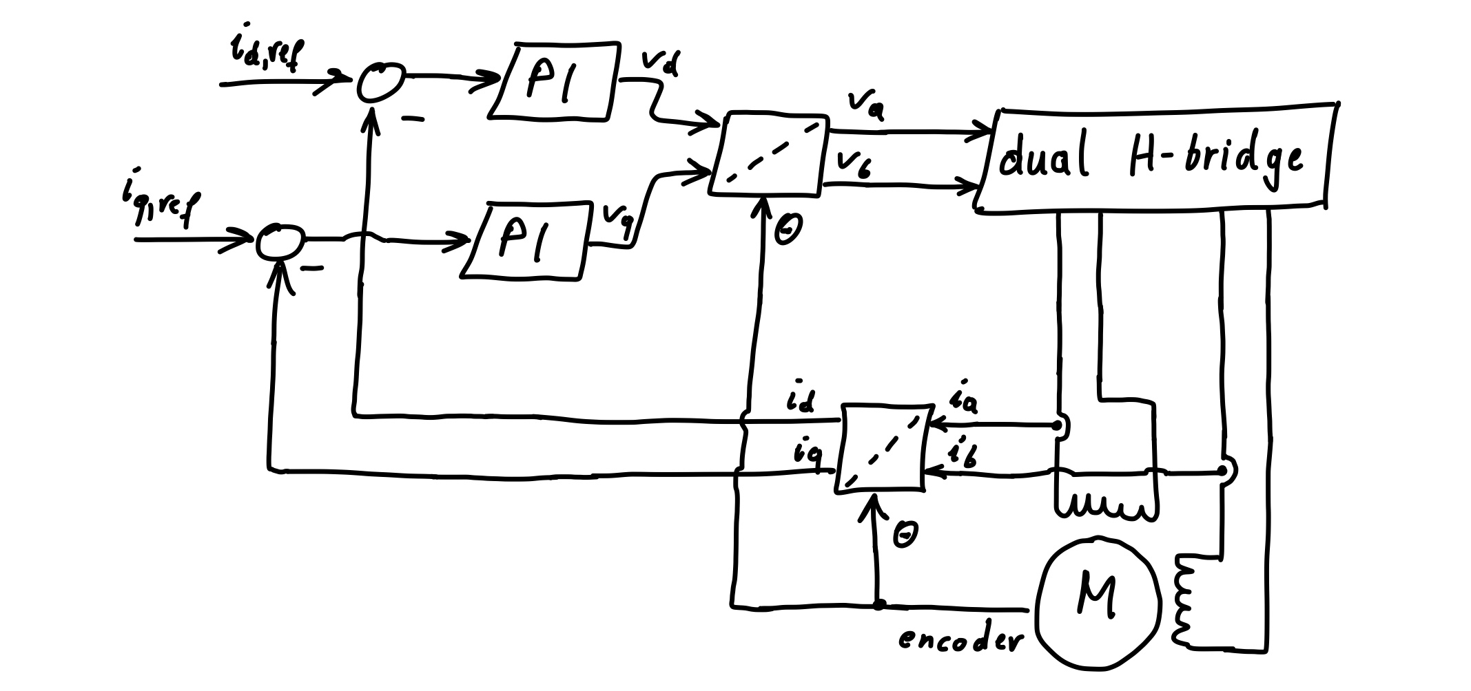
In normal operation, the current \(i_d\) may be held at zero by choosing \(i_{d,ref}=0\). A nonzero value for \(i_{d,ref}\) may be chosen for so-called field weakening – allowing for higher maximum velocity for a given supply voltage.

In the above block diagram, the currents \(i_a\) and \(i_b\) are measured, from which \(i_d\) and \(i_q\) are calculated via (\ref{eq:current_transformation}). The differences of the reference values \(i_{d,ref}\) and \(i_{q,ref}\) and the currents \(i_d\) and \(i_q\) are fed into the PI controllers, which calculate the voltages \(v_d\) and \(v_q\). Via the inverse of (\ref{eq:input_transformation}), the voltages \(v_a\) and \(v_b\) are calculated, which are applied to the motor phases via a dual H-bridge. (The H-bridge is actually not part of the actual control strategy but rather part of a practical implementation of the latter.) The torque generated by the motor is (neglecting the detent torque) given by \(K_mi_q\). The above control scheme, thus allows for controlling the torque of the motor. This torque control loop could be used as part of a velocity control loop with an additional superordinate PI controller, and the resulting velocity control loop could be used as part of a position control loop, e.g. with an additional superordinate P controller.

The above block diagram in Figure 2 is similar to typical block diagrams for FOC of three phase permanent magnet synchronous motors. But here, no Clark transformation is needed since we have a two phase system to begin with and instead of a three phase inverter implementing a SVPWM, each of the two phases of the stepper motor is driven by a separate H-bridge.

A slightly simpler control strategy is obtained by calculating the reference values \(i_{a,ref}\), \(i_{b,ref}\) from \(i_{d,ref}\), \(i_{q,ref}\), and then using PI controllers directly for the currents \(i_a\) and \(i_b\), see block diagram below (such a setup is used in https://doi.org/10.1109/TMAG.2011.2157956).

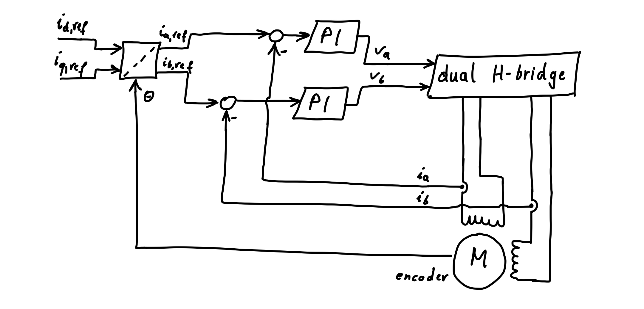
However, this simpler setup comes with a drawback. Namely, even in a steady operating point with constant angular velocity \(\omega\) and load torque \(\tau_L\) (as well as neglected detent torque), and consequently constant \(i_q\), there will be an offset between \(i_{d,ref}\) and \(i_{d}\) as well as \(i_{q,ref}\) and \(i_q\). The reason for that is, that for constant velocity, \(i_{a,ref}\) and \(i_{b,ref}\) are not constant but rather sinusoids with frequency \(Nr\omega/(2\pi)\), which the PI controllers cannot track perfectly. For the control strategy depicted in Figure 2 on the other hand, there will not be an offset between \(i_{d,ref}\) and \(i_{d}\) as well as \(i_{q,ref}\) and \(i_q\) in steady state. The above neglected terms \(N_r\omega i_q\), \(N_r\omega i_d\), \(K_m\omega\) do not mess with that either, since in steady state, these terms are constant and handled by the integrators of the PI controllers. The practical implementation described further below is based on the block diagram in Figure 2.

Discrete Time Current Controllers

For a practical implementation of the control scheme depicted in Figure 2 with a microcontroller, the PI controllers have to be discretized. A priori, there are two possibilities. The first possibility is to design continuos time controllers and then discretize them. The second one is to discretize the plant and then directly design discrete time controllers. When the sampling frequency is chosen sufficiently high, either approach may be used. However, the first approach, i.e. designing a continuos time controller and then discretizeing the controller, actually relies on fast enough sampling, such that the effects of the sampling are negligible. Even if the continuos time controller is designed such that it is able to stabilize the plant, the same controller discretized may fail to stabilize the plant. On the other hand, when first discretizing the plant and then designing a discrete time controller, the effect of the sampling is inherently considered. Although both approaches would probably work here, let us first discretize the plant and then directly designing a discrete time current controller.

Consider again the simplified linear current equations \(\dot{i}_x=\frac{1}{L}(v_x-Ri_x)\). Let \(T_s\) be the sampling period. The discretized model then follows as

\[\begin{align} i_{x,k+1}=e^{-\tfrac{R}{L}T_s}i_{x,k}+\frac{1}{R}(1-e^{-\tfrac{R}{L}T_s})v_{x,k}\,. \end{align}\label{eq:current_model_discrete}\tag{6}\]

I do not go into detail about the derivation. In a nutshell, the difference equation (\ref{eq:current_model_discrete}) describes the behavior of the discrete time system obtained by feeding the continuos time system via a zero-order hold and sampling its output, as depicted in the figure below.

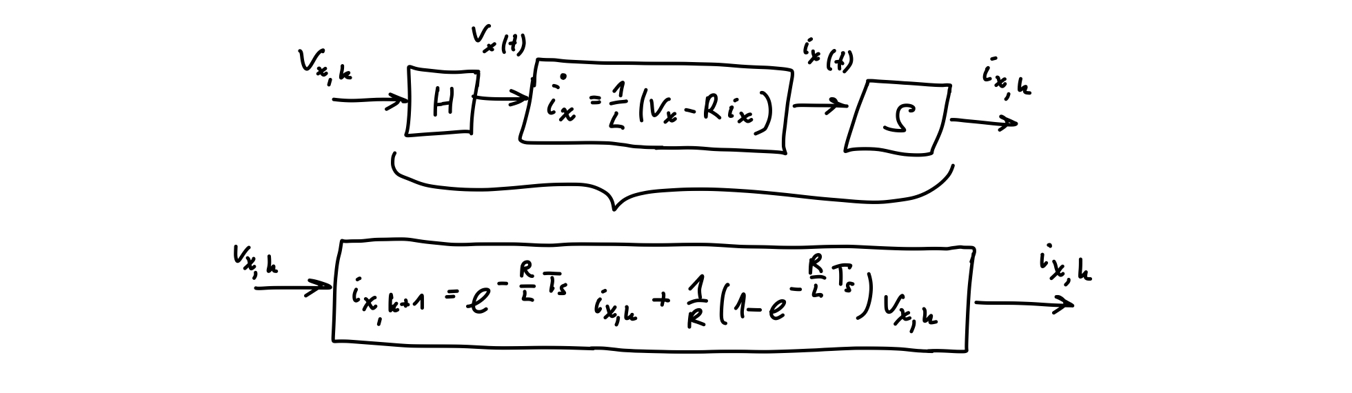
I refer to standard control engineering literature like e.g. Ogata K.: Discrete-Time Control Systems, Prentice-Hall, 1987 for details.

The transfer behavior from the voltage \(v_{x,k}\) to the current \(i_{x,k}\) in terms of a \(z\) transfer function is given by

\[\begin{align} i_{x}(z)=\underbrace{\frac{1}{R}\frac{1-e^{-\tfrac{R}{L}T_s}}{z-e^{-\tfrac{R}{L}T_s}}}_{P_z(z)}v_x(z)\,. \end{align}\]

For the controller, we choose

\[\begin{align} C_z(z)&=V\frac{z-e^{-\tfrac{R}{L}T_s}}{z-1}\,. \end{align}\label{eq:current_controller_discrete}\tag{7}\]

The pole at \(z=1\) of the controller corresponds to a summation (i.e. the discrete time analogue of the integrator in the continuos time PI controller). The zero at \(z=e^{-\tfrac{R}{L}T_s}\) is used for canceling the pole at \(z=e^{-\tfrac{R}{L}T_s}\) of \(P_z(z)\). With this controller, we thus obtain

\[\begin{align} L_z(z)&=C_z(z)P_z(z)=\frac{V}{R}\frac{1-e^{-\tfrac{R}{L}T_s}}{z-1}\,, \end{align}\]

and the closed-loop behavior

\[\begin{align} i_x(z)&=\frac{L_z(z)}{1+L_z(z)}i_{x,ref}(z)=\frac{\tfrac{V}{R}(1-e^{-\tfrac{R}{L}T_s})}{z-1+\tfrac{V}{R}(1-e^{-\tfrac{R}{L}T_s})}i_{x,ref}(z)\,. \end{align}\label{eq:current_closed_loop_z}\tag{8}\]

For stability, the gain \(V\) of the controller must be chosen such that the pole at \(z=1-\tfrac{V}{R}(1-e^{-\tfrac{R}{L}T_s})\) is located within the unit circle, i.e. \(\vert 1-\tfrac{V}{R}(1-e^{-\tfrac{R}{L}T_s})\vert<1\). In the figure below, step responses for the pole locations \(\{-0.5,0,0.5,0.75\}\) are illustrated.

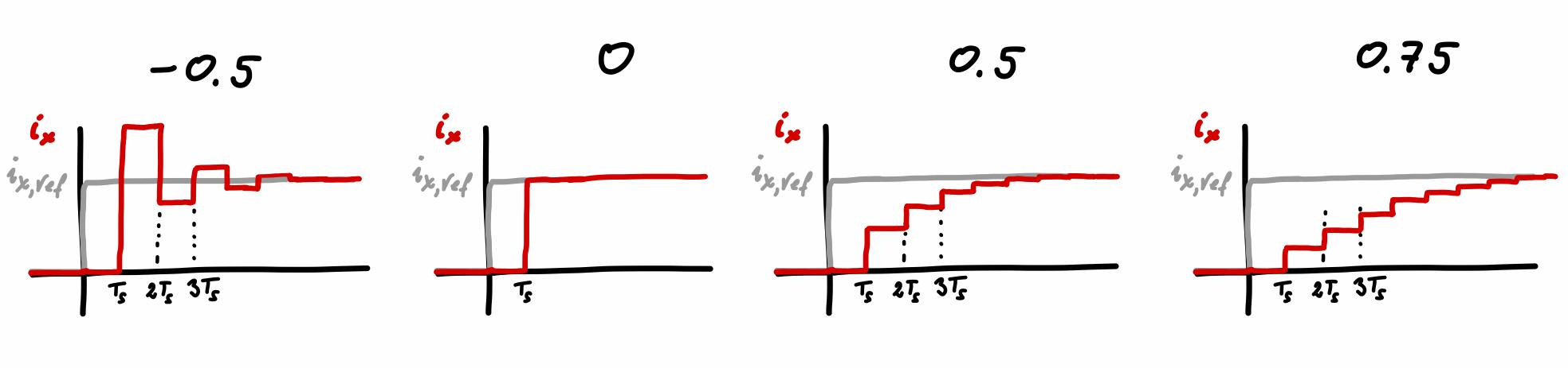
Choosing \(V\) too large, such that the pole is located in the interval \((-1,0)\), is impractical. Locating the pole at \(0\) results in a so-called dead-beat behavior, in which the reference is reached after exactly one sampling period. The smaller \(V\), and consequently, the closer the pole gets to \(1\), the slower is the response. (The closed loop behavior (\ref{eq:current_closed_loop_z}) is of course again only approximate due to the neglected coupling terms which are present in the actual current equations.)

The discrete time controller (\ref{eq:current_controller_discrete}) can easily be implemented on a microcontroller via its difference equation

\[\begin{align} v_{x,k}&=v_{x,k-1}+V(e_{x,k}-Ee_{x,k-1})\,, \end{align}\label{eq:current_controller_difference_eq}\tag{9}\]

where \(e_{x}=i_{x,ref}-i_x\) and \(E=e^{-\tfrac{R}{L}T_s}\). (In the implementation, \(v_{x,k}\) is clipped between \(\pm V_{supply}\). Using the clipped value in further evaluations of the difference equation prevents the discrete time analogue of integrator windup.)

Practical Implementation

Hardware

For testing the control strategy in practice, I came up with the driver board in Figure 6 below.

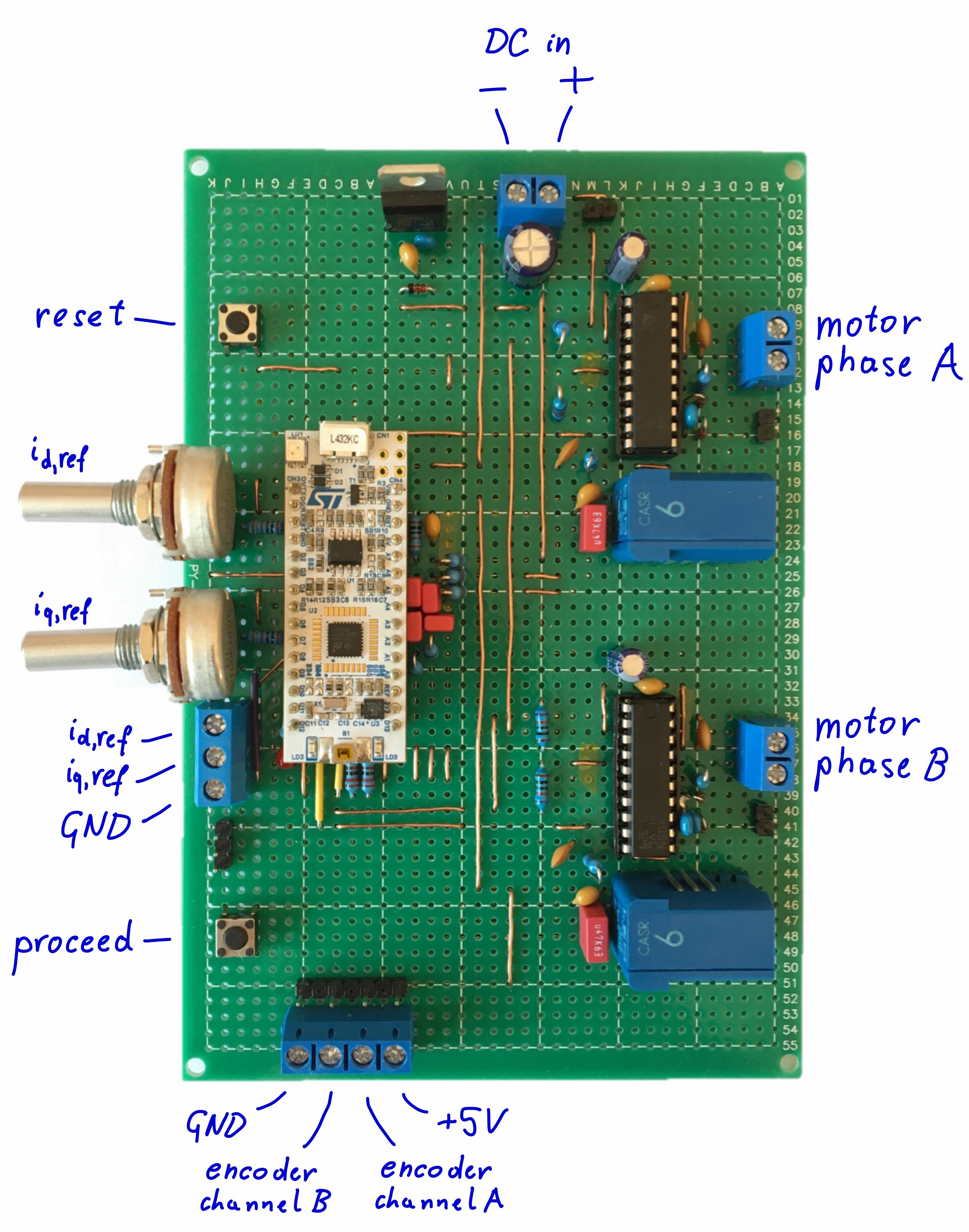
The main components are:

• NUCLEO-L432KC microcontroller board
• L6205 dual H-bridge ICs
• LEM CASR 6-NP current sensors

A detailed schematic of the driver board can be seen below.

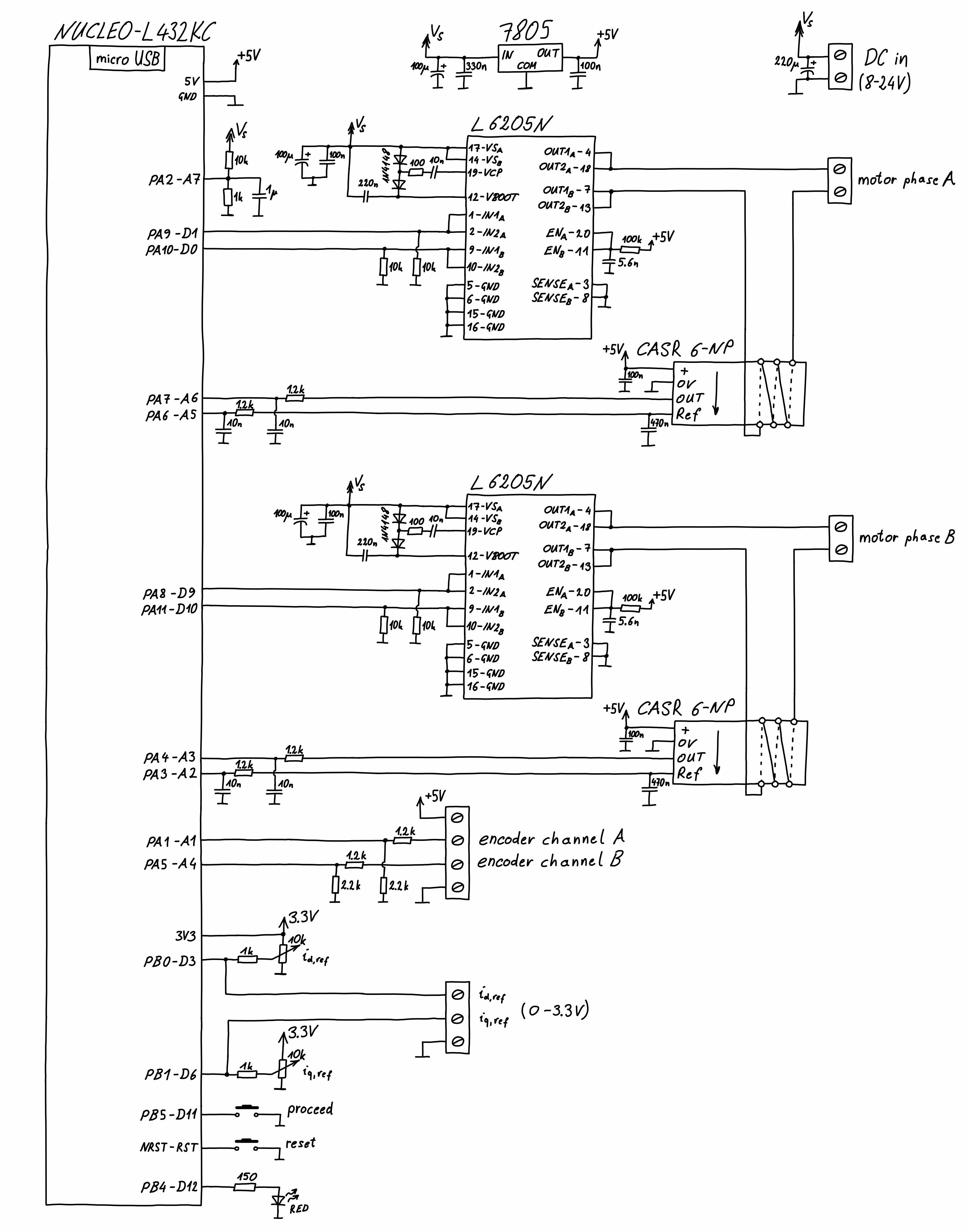
Before connecting the NUCLEO-L432KC microcontroller board via the USB connector to a PC (for programming or debugging), the driver board needs to be supplied with \(8\) to \(24\,\mathrm{V}\) via the DC input screw terminal, otherwise, the microcontroller board may gets damaged! A 7805 voltage regulator generates \(5\,\mathrm{V}\) from the DC input. From these \(5\,\mathrm{V}\) (part of) the NUCLEO-L432KC microcontroller board is supplied via the +5V pin, and also the current sensors and an encoder connected to the corresponding screw terminal are supplied via this \(5\,\mathrm{V}\) regulator. With the default configuration of the solder bridges on the NUCLEO-L432KC microcontroller board, the target STM32 microcontroller (STM32L432KCU6U) does not run unless also the on board ST-LINK is powered (the ST-LINK is not supplied via the +5V pin of the microcontroller board). The reason for that is, that the NRST pin of the target microcontroller is held low by the ST-LINK when the latter is not powered. When the microcontroller board is connected to a PC via the USB connector, the ST-LINK receives power and the target microcontroller can run. In order to run the board without an USB connection, there are two simple solutions: 1. Power the ST-LINK via the Vin pin (according to the data sheet, this pin accepts \(7-12\,\mathrm{V}\), though, according to contributions on the https://community.st.com forum, \(5\,\mathrm{V}\) on this pin also work, which I was able to confirm with my board). 2. Another solution is to remove the solder bridge SB9 on the NUCLEO-L432KC microcontroller board. This way, the NRST pin of the target microcontroller is disconnected from the ST-LINK. A drawback of the second solution is that reprogramming the target microcontroller may not be possible with SB9 removed (I have not tested that). In my opinion, the simplest solution to run the board without an USB connection is to use a jumper wire from the +5V pin to the Vin pin.

The two phases of the stepper motor need to be connected via the screw terminals on the right hand side. Via the screw terminals on the bottom in Figure 6, a quadrature encoder coupled with the motor shaft needs to be connected. The voltage dividers formed by the \(1.2\,\mathrm{k\Omega}\) / \(2.2\,\mathrm{k\Omega}\) resistors (see schematic in Figure 7) allow for directly connecting an encoder which outputs \(5\,\mathrm{V}\) signals. Though, an encoder which outputs \(3.3\,\mathrm{V}\) signals can still be used with these voltage dividers. It is crucial that the motor and the encoder direction match, i.e. a clockwise rotation of the motor must be detected as a clockwise rotation by the encoder. Otherwise, the encoder signal lines or the motor phases or the polarity of one motor phase need to be swapped. The reference values for the motor currents \(i_d\) and \(i_q\) need to be supplied via the screw terminal on the left as an analog voltage between \(0\) and \(3.3\,\mathrm{V}\) (the input voltage range \(0\) to \(3.3\,\mathrm{V}\) corresponds to the current range \(-I_{max}\) to \(+I_{max}\) with \(I_{max}\) set in the code). The board must be powered before applying voltage to this screw terminal. When nothing is connected to this screw terminal, the reference values can be set via the potentiometers (center position corresponds a reference value of \(0\,\mathrm{A}\)). Next to all the screw terminals I soldered pin headers, which eases probing the corresponding signals with an oscilloscope and proved to be very useful for debugging.

The button on the top is just a reset button (I accidentally broke the tiny reset button of the NUCLEO board). The other button is used to initiate the encoder alignment (see below) and afterwards to initiate the execution of the actual control algorithm.

The voltage applied to a motor phase depends on the supply voltage and the duty cycle of the corresponding PWM signal. Since the board may be supplied with any voltage in the range \(8\) to \(24\,\mathrm{V}\), the analog input A7 is used for monitoring the supply voltage. This way, the duty cycle which is needed to apply a certain voltage to a motor phase can always be calculated. The red LED next to the lower left corner of the NUCLEO board lights up when the duty cycle of a PWM signal reaches \(100\%\), i.e. when actuator limits are hit.

Instead of two L6205 H-bridge ICs, a single one could be used. The L6205 contains 4 half bridges, which all can be controlled individually. These four half bridges may be used to form two H-bridges (in this configuration, one L6205 would suffice here). However, the individual half bridges of one L6205 can be paralleled in oder to form a single H-bridge or only a single half bridge with correspondingly higher load current capabilities (see data sheet for details). In the above driver board, two L6205 are used, one for each of the two phases of the stepper motor, with each of them configured as a single H-bridge. For even higher current capabilities, one may use four L6205’s, each configured as a half bridge. (In any of these three possible configurations, we end up with two H-bridges, controlled via four signals, namely one control signal for each of the four half bridges.)

In the above schematic, there is no distinction made between power ground and signal ground. In the actual layout of the board, it is of course crucial to not use ground connections which carry load current also as return paths for signals. In particular, the power ground connection between the negative of the DC input, the SENSE pins of the L6205 and the decoupling capacitors of the L6205 must not be used as return path for any signals. The simplest way to avoid interferences due to shared return paths, in particular when working with prototyping boards which do not feature a ground plane, is to use star grounding. Furthermore, interference of sensor signals by PWM signals should of course be held as low as possible.

Firmware

At a high level, the program running on the microcontroller executes the following steps:

• initialization of sin and cos lookup tables
• calculation of current controller parameters from the motors resistance and inductance
• initialization of peripherals (timers, ADC, GPIOs)
• encoder alignment
• in an endless loop:
  • read encoder
  • read the currents \(i_a\) and \(i_b\) (current sensors)
  • calculate \(i_d\) and \(i_q\) (via (\ref{eq:current_transformation}))
  • read the set points \(i_{d,ref}\) and \(i_{q,ref}\)
  • calculate \(v_d\) and \(v_q\) via the current controller difference equations (\ref{eq:current_controller_difference_eq})
  • calculate \(v_a\) and \(v_b\) (via the inverse of (\ref{eq:input_transformation}))
  • read the supply voltage
  • set the PWM duty cycles for generating the calculated voltages \(v_a\) and \(v_b\)
  • wait for the remainder of the control algorithm sampling period

For programming the microcontroller board, I used the STM32CubeIDE and C as programming language. All the source code can be found in the github repository https://github.com/conrad-gst/stepper-motor-foc When writing the code, I did not focus on efficiency, but rather on simplicity. In particular, all calculations are done in floating point and in SI units. E.g. the analog voltages from the current sensors, which after the analog-to-digital conversion are 12 bit values, are converted to floating point values which represent the current in amperes. Via the control algorithm, the phase voltages are calculated in volts, which are then converted to a PWM duty cycle. Such conversions are not efficient an in fact not necessary. It would be more efficient to implement the control algorithm such that there is directly a duty cycle calculated from the 12 bit values coming from the ADC. However, debugging and maintaining such code would be very tedious.

After all the initializations, i.e. before the encoder alignment, the program is paused and the “proceed” button needs to be pressed in order to initiate the encoder alignment. For aligning the encoder, a current is passed through motor phase A while the current through phase B is held at zero. This is done for several seconds, the position in which the rotor settles defines the zero position in which the d-axis and the a-axis are aligned. After the alignment phase, the “proceed” button needs to be pressed again in order to enter the endless loop, i.e. to initiate execution of the actual control algorithm. The program being paused and waiting for the “proceed” button to be pressed is indicated by the green LED on the NUCLEO board. The red LED connected to pin PB4 (see schematic in Figure 7) is used for indicating when a current controller hits the voltage limit of \(\pm V_{supply}\). Furthermore, the red LED lights up when an over current is detected (in this case, the outputs are set to zero and a reset is required). To safely shut down the system one has to press the reset button.

Demonstration

All the following demonstrations were done with a stepper motor from ACT Motor GmbH with the type designation 23SSM6440-EC1000. It is a hybrid stepper motor with \(1.8^\circ\) step angle and it is fitted with a quadrature encoder with \(1000\) steps per revolution (the effective resolution is thus \(4000\) steps per revolution). According to its data sheet, it has a phase resistance of \(R=0.4\,\mathrm{\Omega}\) and a phase inductance of \(1.2\,\mathrm{mH}\). It can handle a phase current of up to \(4\,\mathrm{A}\). In all experiments, the driver board was supplied with \(12\,\mathrm{V}\). I do not have professional testing equipment which would allow me to precisely characterizing the behavior of the motor when controlled with the implemented FOC scheme. The demonstrations below are just rudimentary demonstrations of the behavior and not scientific tests.

Constant Torque

In this demonstration, I set \(i_{q,ref}\) to a constant value via the corresponding potentiometer (roughly \(1\,\mathrm{A}\)). This should result in a constant torque \(K_mi_q\) acting on the rotor (up to the detent torque), regardless of the rotor position or speed, which indeed seems to be the case – the rotor can be pushed around but always accelerates in the same direction when released.

Torque vs. Current

In steady state with zero velocity and when neglecting the detent torque and the static friction, according to the model (\ref{eq:stepper_motor_dq}), the torque of the motor is given by \(\tau_L=K_mi_q\). In this test, I measured \(\tau_L\) for different values of \(i_q\) and estimated \(K_m\) from these measurements. The parameter \(K_m\) is not directly specified in the motors data sheet (but it can be calculated from specified parameters, see below). The setup can be seen below.

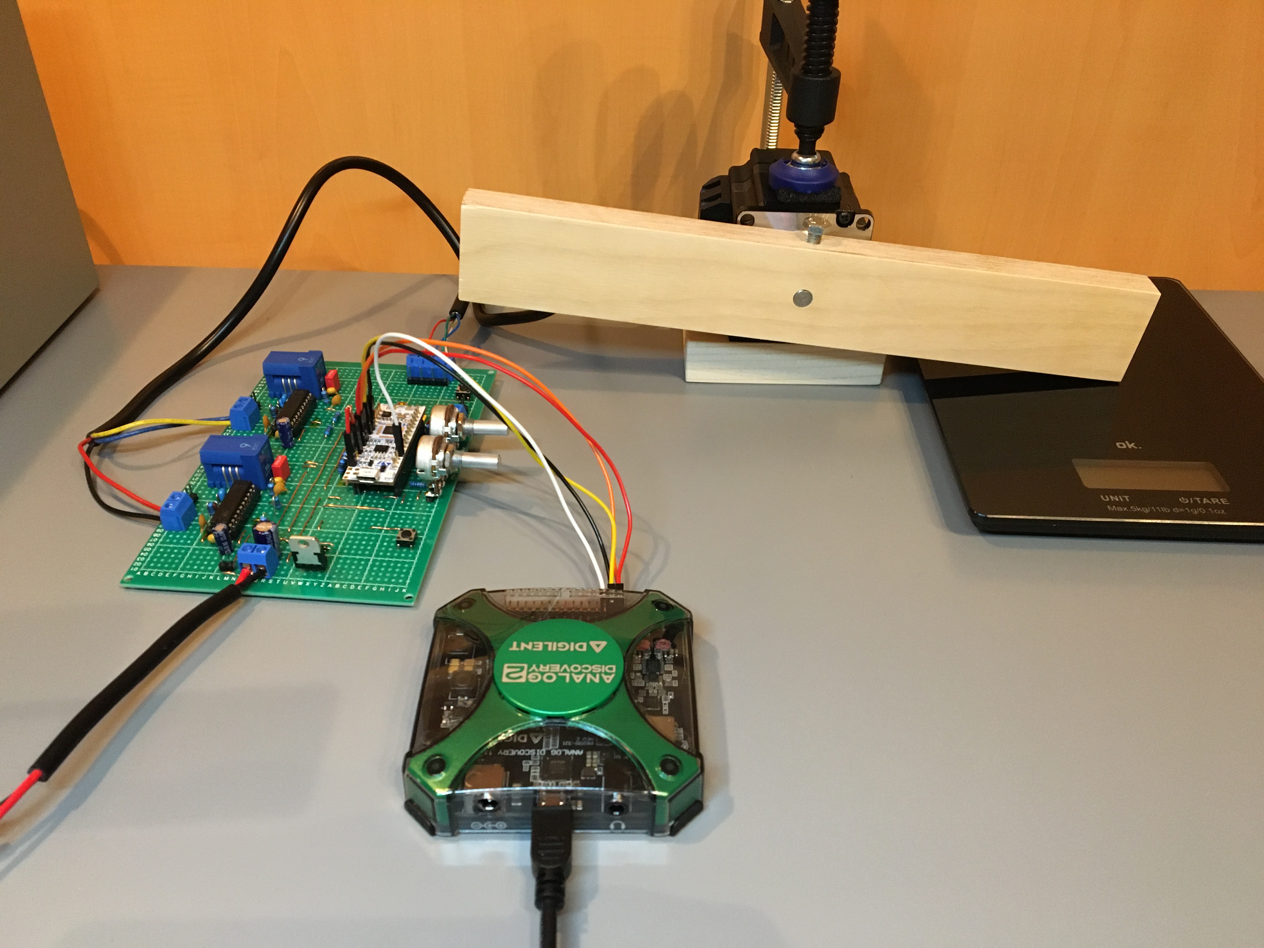
I used an Analog Discovery 2 for measuring \(i_q\). For that, the output signals of the two current sensors were measured with the two scope channels of the Analog Discovery 2. Under the assumption that \(i_d\equiv 0\), it follows that \(i_q=\pm\sqrt{i_a^2+i_b^2}\). The AD2 can easily be set up for calculating \(i_q\) from the sensor signals and trace it. The torque is obtained from the force pressing down on the kitchen scale and the length of the lever.

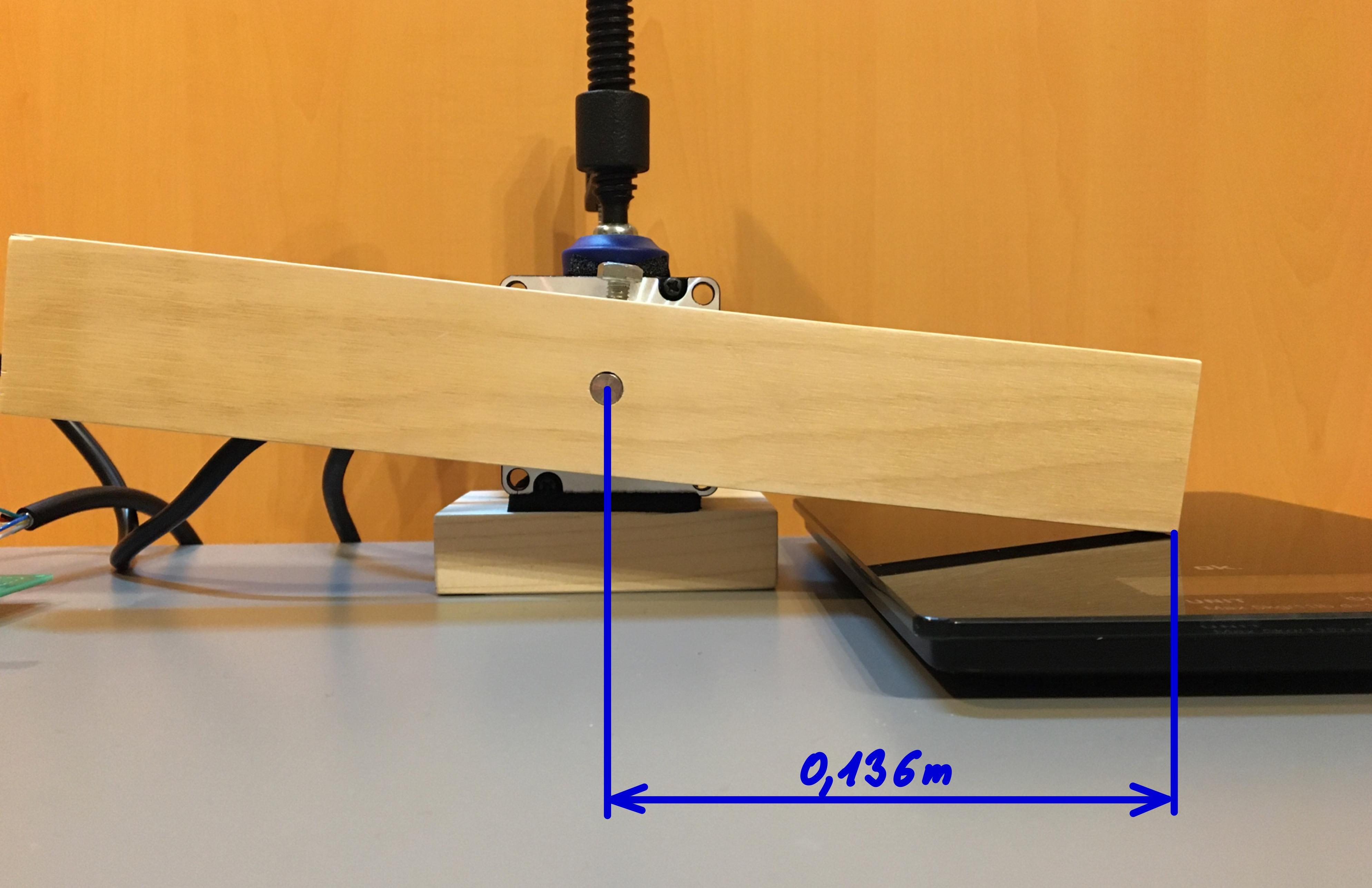
Unfortunately, the measurements which I obtained with this setup were not very reproducible. In a next attempt, I shortened the effective length of the lever from \(0.136\,\mathrm{m}\) to \(0.049\,\mathrm{m}\) with a wood screw as can be seen below.

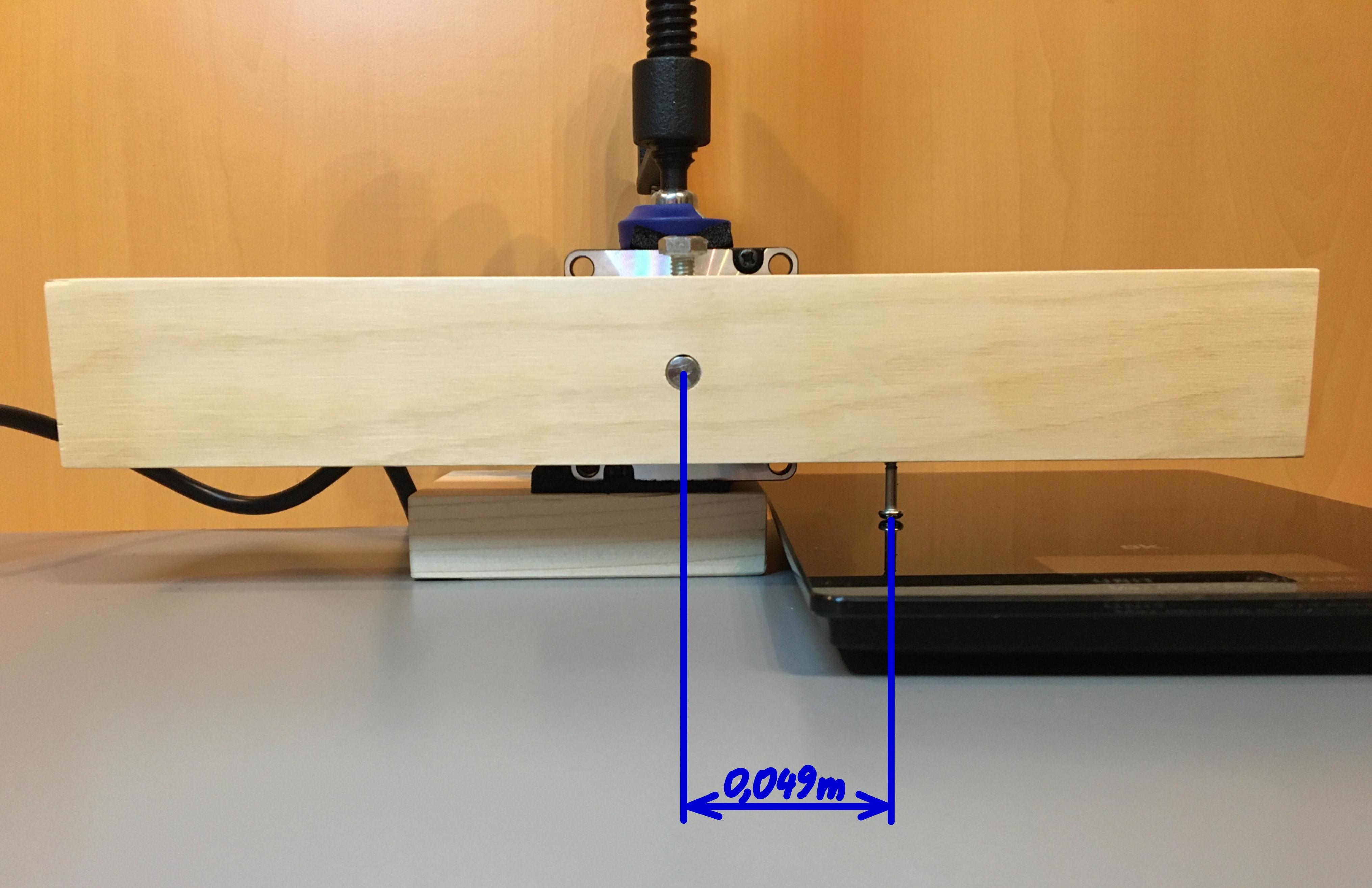
With this setup, I achieved much more reliable results. The obtained measurements are illustrated below.

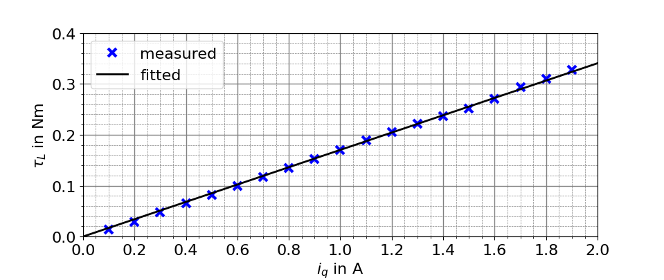
For estimating the motor parameter \(K_m\) from the \(N=19\) current-torque pairs \((i_{q,i},\tau_{L,i})\), I fitted a line \(\hat{K}_m i_q\) to this data with the slope \(\hat{K}_m\) determined such that the sum of the squares of the errors is minimized, i.e. such that \(\sum_{i=1}^{N}(\tau_{L,i}-\hat{K}_mi_{q,i})^2\) is minimized (least squares method). The slope of the obtained line is \(\hat{K}_m=0.170\,\mathrm{Nm/A}\).

As already mentioned, the motor parameter \(K_m\) is not specified in its data sheet, but a holding torque of \(1.1\,\mathrm{Nm}\) and a maximal phase current of \(4\,\mathrm{A}\) are specified. Under the assumption that the given holding torque occurs when \(i_a=i_b=4\,\mathrm{A}\) with the rotor aligned for maximum torque, \(K_m\) follows as \(K_m=1.1/\sqrt{4^2+4^2}=0.194\,\mathrm{Nm/A}\). This value is not too far from \(\hat{K}_m=0.170\,\mathrm{Nm/A}\) calculated above.

Interestingly, a detent torque, which in the motors data sheet is specified with at most \(0.04\,\mathrm{Nm}\) does not really show up in the measurement data depicted in Figure 11. Maybe, the angle \(\theta\) at which the lever touches the scale is accidental such that the detent torque term \(K_D\sin(4N_r\theta)\) (see (\ref{eq:stepper_motor_ab})) is very small. I also tried to measure \(K_D\), i.e. the amplitude of the detent torque. For that, I held the motor in my hand, very carefully pressed down on the scale with the lever and read the scale just when the rotor started to turn. Thereby, I determined \(K_D\approx 0.023\,\mathrm{Nm}\), which is indeed much lower than the \(0.04\,\mathrm{Nm}\) from the data sheet (although my measurement should actually also include some static friction). (When \(K_D\) and \(K_m\) are known, the detent torque could be compensated by adding \(\tfrac{K_D}{Km}\sin(4N_r\theta)\) to \(i_{q,ref}\).)

Rotary Spring Emulation

For this demonstration, I slightly modified the program running on the microcontroller. I defined \(i_{q,ref}=-k\theta\) with \(k=0.8\,\mathrm{A/rad}\). This position feedback emulates a rotary spring. With \(\hat{K}_m=0.170\,\mathrm{Nm/A}\) from above, the spring constant of this rotary spring follows as \(c=k\hat{K}_m=0.136\,\mathrm{Nm/rad}\). Neglecting the detent torque and assuming that \(i_d\equiv 0\) and \(i_q\equiv i_{q,ref}\), the mechanical subsystem is then described by the model

\[\begin{align} \dot{\theta}&=\omega\\ \dot{\omega}&=\frac{1}{J_r+J_{lever}}\big(-c\theta-B\omega-\tau_L\big)\,, \end{align}\]

where \(J_r\) is the moment of inertia of the motors rotor (according to the data sheet, we have \(J_r=300\,\mathrm{gcm^2}=3\cdot 10^{-5}\,\mathrm{kgm^2}\)) and \(J_{lever}\) is the moment of inertia of the attached wooden lever (neglecting the screw with which it is attached to rotor, we have \(J_{lever}\approx 9.1\cdot 10^{-4}\,\mathrm{kgm^2}\)). In the video below, the rotor is pushed and then released. When released, we have \(\tau_L=0\) and see a damped oscillation. This damped oscillation should thus be a solution of

\[\begin{align} \dot{\theta}&=\omega\\ \dot{\omega}&=\frac{1}{J_r+J_{lever}}\big(-c\theta-B\omega\big)\,. \end{align}\label{eq:stepper_motor_rotary_spring}\tag{10}\]

From the general solution of (\ref{eq:stepper_motor_rotary_spring}), formulas for determining \(c/(J_r+J_{lever})\) and \(B/(J_r+J_{lever})\) from the period and the rate at which the oscillation decays could be derived. Period and rate of decay could be determined by analyzing the video frame by frame. Thereby, the parameter \(B\), which models friction, could be determined and furthermore, the above estimate for \(K_m\) could be verified.

Conclusion

Although stepper motors are primarily intended for positioning tasks without position feedback from an encoder, fitting them with an encoder gives new possibilities for controlling them. The field oriented control scheme described here allows for controlling the torque of the motor and this torque control loop may be used in a cascade speed or position control. The described control scheme essentially turns a stepper motor into a relatively inexpensive servo drive, useful e.g. for hobby robotics projects. An advantage of torque controlled stepper motors over torque controlled DC motors of similar size is that they can produce a much larger torque, which may eliminate the need for a gearbox.