Magnetic Levitation

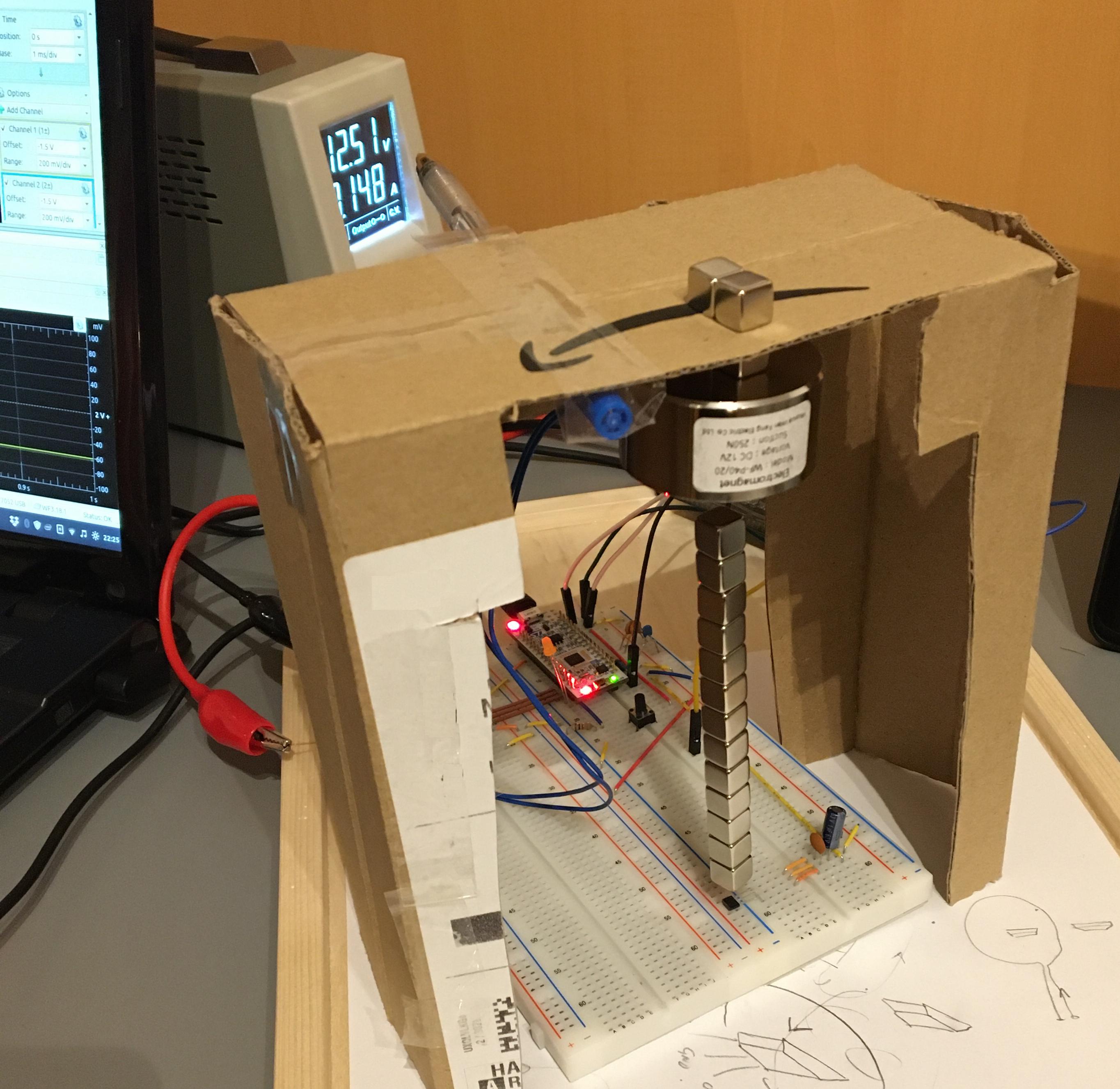
This article is about a crude magnetic levitation experiment quickly thrown together on some weekend. The purpose of the setup is to let a stack of \(10\,\mathrm{mm}\) neodymium magnet cubes hover under an electromagnet. In order to accomplish this, a PID feedback loop has been used. The setup can be seen in the figure below. The main components are:

• NUCLEO-L432KC microcontroller board
• TB6612FNG H-bridge ic breakout board
• Electromagnet
• some \(10\,\mathrm{mm}\) neodymium magnet cubes
• 49E linear Hall-effect sensor
• Breadboard
• Frame made of cardboard, sticky tape and a ballpoint pen for extra rigidity of the construction 😅

I do not have a data sheet for the electromagnet. It has a diameter of \(40\,\mathrm{mm}\), a hight of \(20\,\mathrm{mm}\), and it is rated for \(12\,\mathrm{V}\) and for holding a load of \(25\,\mathrm{kg}\).

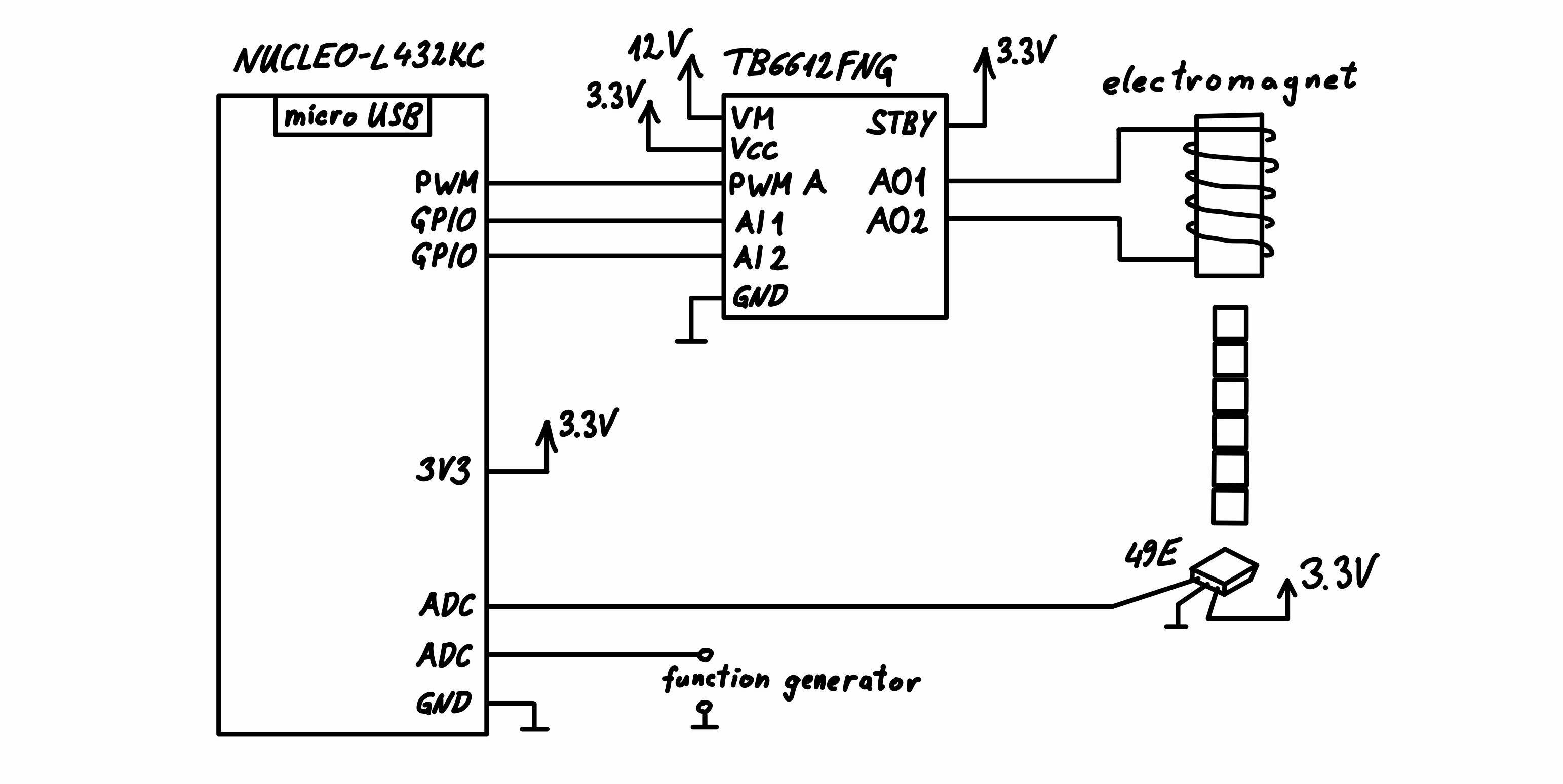
A simplified schematic of the setup can be seen in the figure below. The output voltage of the linear Hall-effect sensor below the stack of neodymium magnet cubes is related to the distance of these magnets from the sensor, thus providing a means of measuring the position of the magnets. The output signal of the Hall-effect sensor is feed into an ADC pin of the NUCLEO-L432KC microcontroller board. The microcontroller runs a PID control algorithm (more on that later). A function generator connected to another ADC pin provides the set point for the control loop. Based on the set point signal and the signal coming from the Hall-effect sensor, the microcontroller computes the voltage to be applied to the electromagnet via a PID algorithm. To actually apply the calculated voltage, the H-bridge is feed by a \(32\,\mathrm{kHz}\) PWM signal with the corresponding duty cycle.

The transfer function of a PID controller with realization pole is given by

\[\begin{align} C(s)&=\frac{u(s)}{e(s)}=P+I\frac{1}{s}+D\frac{s}{1+\tfrac{s}{\omega_0}}\,. \end{align}\]

(The larger \(\omega_0\), the larger is the frequency up to which the derivative term indeed behaves like a differentiator.) For an implementation in a microcontroller, the transfer function needs to be discretized. Here, following https://www.scilab.org/discrete-time-pid-controller-implementation, the backward Euler method has been used for the discretization. In a nutshell, we simply have to substitute \(s=\tfrac{z-1}{T_sz}\), which yields the \(z\)-transfer function

\[\begin{align} C_z(z)&=P+I\frac{T_sz}{z-1}+D\frac{\omega_0(z-1)}{(1+\omega_0 T_s)z-1}\,, \end{align}\]

where \(T_s\) is the sampling time. In my setup, the control algorithm running on the microcontroller is a realization of this \(z\)-transfer function in form of a difference equation, augmented by an integrator windup protection. The control loop runs at a frequency of \(2.5\,\mathrm{kHz}\), i.e. the sampling time is \(T_s=400\,\mathrm{\mu s}\).

Experimental Results

In the video below, the function generator voltage (i.e. the set point of the control loop) has been set to a constant value. The stack of cube magnets levitates at a constant height.

Besides a constant set point, I also tried a low frequency sinusoid, which is nicely tracked. The cube magnets dangle up and down such that the voltage of the Hall-effect sensor tracks the low frequency sinusoid coming from the function generator.